CGMatter masterfully bridges the gap between complex calculus and visual art by turning Blender's nodes into a functional physics engine. This project proves that even the most rigorous fluid dynamics can be democratized through creative visual programming.
Install our extension to search inside any video instantly.
I made a fluid solver with nodesAdded:
I'm very proud of these fluid simulations which also include smoke by the way that's also a fluid because it is mine. I made this geometry node my fluid solver. Actually it is my iterative pson solver on a collocated grid and a vector. What? It only gets mathier from here. This video is sponsored by Squarespace and we're going to talk about that later. If I have a velocity grid saying where things move or flow, I can put a little ink or a little smoke and it will follow it. So when it comes to fluid solvers, if you can make a velocity grid saying where should the fluid flow, you're golden.
Everything else comes from that. The thing is, you can't use any velocity grid you want. For example, here's a velocity grid and I moved the smoke along it and it behaves very, very weirdly. This is because fluids are incompressible. You see how there's areas where things compress or expand?
That shouldn't happen. We say that it is divergence free, meaning it can't expand or contract. Now, Helmhot's decomposition tells us this, which is a very confusing way to say any vector field pretty much can be split into a curl-free component and a divergence free component. A second fact is that the gradient of a scalar field is always going to be curl-free. But interestingly, it goes both ways.
Meaning, if you have a curl-free field, it is the gradient of some scalar potential. And here comes the magic. If I take the divergence of both sides, I have the divergence of our vector field is equal to the divergence of this weird thing plus what do you think the divergence of a divergence free field is? It's zero. And what we're left with is something that is called a pson equation. That's a well-known problem.
Let's expand out the gradient of the scaler. take the divergence of this and then just swap things around. If you do the math, you're going to end up with this equation. And what this tells us, here's the key insight. We can find our scalar function by iteratively applying this process. For each cell, I look at its neighbors. I add them together, subtract a divergence with hide by 6. Do this over and over and over and over again. I'm going to converge to this scaler that we're looking for, which we can take the gradient of, subtract it away from the vector field, and then we get the divergence free part, which is how a fluid behaves. So, so that's the theory. In practice though, let's take this one step at a time. So we know we need a grid to work on. On this grid, I need a few things. So this is my grid topology and I want to track the velocity of the fluid. Maybe the density and then also the scalar fee function.
In general, a vector and then two different scalar fields. Velocity, density, fe. Then all of these get sent through a simulation loop. Let's just connect all these bad boys over here.
And now let me describe how the simulation works. We start with a velocity field saying how will the fluid move? We then advect or in other words apply this velocity not only to the density field saying fluid move this way but we actually advect the velocity itself. This is the conservation of momentum. Once you have that you add forces like gravity. We know the velocity is supposed to be divergence free. So we do this whole correction pan solve step. That's what it was all for.
I'm going to advect the velocity along itself with a time step of dt. By the way, if you ever see me use a node you do not have, it is available for free at cgmatter.com. No sign up, no nothing.
And I'm going to advect the density grid. A float density grid along the velocity with this dt. And look at that.
We're done with adction. That part's done. Next, what we do is I add forces.
Let's add gravity. So - 9.8. And then a scale of dt. Don't add the whole force on every frame, but just based on the time difference. So one dt step, another dt. Boom. And now the last step was taking this new velocity field and defunking it. Getting rid of the divergence. So, I'm going to throw in a repeat zone cuz that equation I gave you is something we apply iteratively.
Remember, I'm iterating over the scalar field that we invented called feet. Not feet. It's not feet. It's feet. What do we do inside of this loop? Well, like I said, you have to add the neighboring cells. So, in 3D, there's a left, right, front, back, up, down. For the sake of convenience, I already turned this into a nice little node group. Put in a grid and you get, you know, your right, left, front, back, blah, blah, blah. So, I didn't want to make this. Okay, you can get that for free. So, we take our feed.
We add all of these together. So I'm going to add all of these together. Then we are going to subtract the divergence of the vector field times this weird h squ. The divergence is simple. I can just take this calculate the grid divergence and we're done. But remember we have to do this h squared thing. h is the gap between the voxal cells. In other words, the size of a voxal cell.
We know our cube grid topology is a cube minus one on the x plus one on the x and same for all the other dimensions. It is going to have a span of two each individual cell that this is composed of. Then remember there are 32 of these.
They are going to have a length of 2 / 32. 2 / 32. Square it. Multiply these two together. And this whole thing is what I subtract away. That becomes our feed. This tutorial is sponsored by Squarespace, the best place to make a website online. If you head over to cgmatter.com, you can see the website that I have made. Then you can see I made it like highly customized. And Squarespace makes that super easy with a bunch of features. So first of all, I really like that Squarespace has a integrated payment system. I partly use my website to have like a membersonly area with exclusive posts. Second of all, there's a built-in asset browser which lets me save files and host them and then I can share them whether they be images, videos, whatever. Then thirdly of all, there is direct AI integration in the Squarespace editor if you want to use it. This makes filling out content super easy, especially if it's like predictable like documentation or what have you. Head over to Squarespace. There's a 14-day free trial. You can go make a website and when you are ready to launch, you can use this link below in the description.
It's also written out here to save 10% off your first purchase of a website or domain. And again, you have that 14-day free trial. Just to reiterate, we have this equation that if we plug in over and over and over again, we can solve for this fee, which will help us get the divergence free part. And again, we're assuming this has a resolution of 32, otherwise you need to update this.
You're going to see I added a ghost cell option. The reason for this is if you are on the edge of a grid, for example, you're all the way on the left side, you don't have a neighbor on your left. What ghost cells does is it says if you do not have a neighbor, in other words, it is a ghost, either set it to zero or set it to yourself. If I don't have a neighbor, I'm just going to use my own value. Anyways, remember this fee isn't like what we want. At the end of the day, we want to use this to subtract away the curl-free part. We take the gradient of this, then take our magical vector field that is funked and we subtract away the curl-free component resulting in only the divergence free component. And that is our velocity grid. We view the velocity grid. You're going to see that there's nothing. And this is where it gets a little dicey.
You know, if it wasn't dicey already.
The issue is this advect grid node just behaves weirdly. I don't know how else to put it. That's why I made my own for that uh previous tutorial. After add vecting a grid, we're not just going to take this output, but instead we're just going to write this onto a new grid entirely. Sample this grid. You know, I do want these results, but I want to put this in a different grid. I'm going to use my original cube grid topology.
That's what everything is based off of.
Just going to pass this through and connect this to where it would have been. And now you can see we get this.
It just takes our calculation and says put it back on the same grid. You know, the same idea should apply to our density grid. So, we can use the same field to grid node. Then, let's take that bad boy and connect the density all the way over here to the density. If I now instead look at my density grid, you're going to see nothing. Again, this is because we had no density to begin with. We had nothing to send through the flow. So, our flow is working. Maybe we can just make a little ball of density.
Let's just take the 3D positions in space, take their length, in other words, saying how far are you from the center and check where is this less than some value. Connect that into the density. And you can see we have this little ball that when I click play, it indeed falls. Although it falls right through, but that is good evidence that this is working. I'm going to turn this into kind of like an ellipsoid. So we have a different initial density. It also falls. So whatever density we put in, it just flows along the thing. Wait, wait, wait, just wait a second. I talked about this equation so much and I forgot to divide by six at the end. Remember that? That was part of it. Divide by six. Let's actually like consolidate this. All of this can be considered it can be considered our pson solve where I care about the iterations. That's very important. This whole step over here with the ad vection. Well, it can be just that, right? Add vection. This section right here where we basically Oh, give me more battery. No wonder my computer keeps crashing. This part over here can be add forces. Okay, big improvement. Now, I want to mention this like falling through problem. Really, all we want to do is we want to say when it's like about to fall through, in other words, it's near the boundary, the velocity shouldn't be allowed to just like pass right through. We need to kind of kill that direction and only keep the tangential component. When we're near this wall over here, the velocity can't penetrate, but instead it kind of goes upwards. I need to charge my laptop.
Okay, I'm I'm back. I'm back. Let's finish her up. Like I said, on the boundary, we need to split the uh I don't know what I'm doing. Split the vector field into its normal and tangential components. Easy enough.
Before the adction step, I'm going to do this like velocity splitting. And then everything continues as per the us. I have a node that again you can have for free. It's called split vector to components. What it basically does is it takes a vector like for example the velocity grid. It takes in a direction and it can remove that component. Keep everything perpendicular to that or everything in that direction. I can't just plug this in immediately because this is a grid quantity. I am going to sample the grid. Evaluate this vector in which direction. Well, it depends if I'm on the left, right, up, down boundary.
Here's kind of like a cheat. I'm going to make a cube. What I like about that is now finding which normal you're looking for. So, for example, if I'm right here, you just look at the nearest surface to the cube and then you evaluate its normal. For this cube, I'm going to get the nearest surface statistics. This is just a note I did that extracts the normal, the position, all these things. So, for the cube, I want to know its normal direction. This is what we're going to cancel out. And I'm not just going to replace this in right here, which has to be a grid. But I need to do this correction only when we're at the boundary. In other words, the distance to the walls of the cube is really, really tiny. Let's look at the distance when it's less than one cell wide. That was going to be 2 / 32. going to mix a vector where by default we have the velocity and under this distance condition we're going to use this perpendicular component. If you're close to the wall, don't go through it.
Instead, go up or down. Just avoid it.
We need this to be a field. Let's just do our good old field to grid. And I'm going to be lazy and just like plug in this velocity grid from here. I don't think it matters. I'm not sure about that though. Anyways, I'm going to plug this in here. We may as well turn into a node group tangential. And now when I play this, it still doesn't work. This just tells me that something is still wrong. I happen to know it's the pressure solve. We have this pan solve.
That is perfectly fine. But once we calculate it, we've completely discarded it. So you can see that this fee in the simulation goes back to zero. Now technically this is fine as long as your iterations are super high. But you may as well say I'm going to solve it. I'm going to go one frame over. The solution is going to be almost the same. And you kind of keep your progress. So what I would recommend is I'm going to take my feet connected there. Now let's see what this does. It does something. It kind of avoids the wall. I think the reason it's behaving so strangely, if I go into the pson solver, remember we're doing a 32x 32x32 grid, but the indexing starts at zero. It's really 0 through 31. Long story short, I think I need to correct this node. So, for now, I think I need to set this to 31. Yeah. And now it's behaving in a way that makes a bit more sense. It's like falling to the ground and then spreading out as much as it can. Now that we generally have the fluid simulator working, the only thing that separates this from a good-looking result is detail level and forces and turbulence. Let's just try adding a force and seeing what happens. We know that we have gravity and we scale it by dt. Instead of this, I'm going to take 9.8 and I'm going to add a sort of turbulence term which I'm just going to use a unnormalized noise texture for.
You can always scale it by a bigger number like 10. And now we're getting something closer to like the dust that comes after like a muzzle flash or something like that. And I should mention the perfect result that we want is achieved by bringing up the pan solves and the resolution. But throughout this whole tutorial, my laptop's been pooping the bed. There's only so much poop one can handle before he uh hangs in the towel. So, get the full version. It's just this, but way better over on my website, cgmatter.com.
Related Videos

Agentforce NOW AMA: Build with React and Salesforce Multi-Framework
SalesforceDevs
490 views•2026-05-28

How agent o11y differs from traditional o11y — Phil Hetzel, Braintrust
aiDotEngineer
450 views•2026-05-28

Re: 🗣️📍theprophedu📍2026 GST 103 CLASS (E-EXAM REVISION)
theprophedu
636 views•2026-06-04

WEB TECHNOLOGIES UNIT-2 | Degree 4th sem BCOM Computers web technologies unit-2 full explanation💯✅
LearnwithSahera
1K views•2026-05-29

More tests are always better? How to use AI to identify tests that bring little value
Alliance4Qualification
335 views•2026-05-29

Search Algorithms Explained in 60 Seconds! 🤖💨
samarthtuliofficial
218 views•2026-06-01
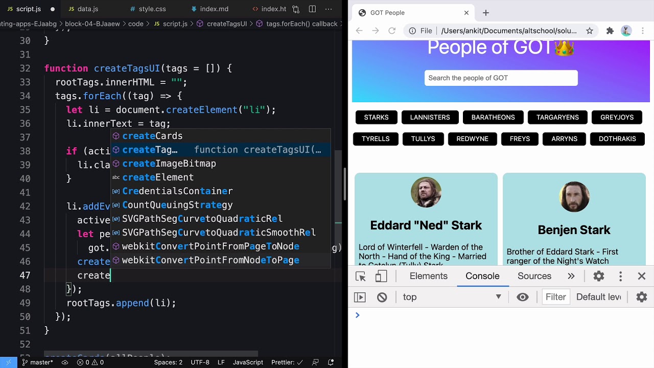
People of Game of Thrones using JavaScript DOM
AltCampus
296 views•2026-05-30

Instagram accounts got PWNed
EricParker
13K views•2026-06-03


