This project provides a lucid, hands-on masterclass in signal processing by turning abstract Fourier transforms into a functional communication bridge. It’s a refreshing return to engineering fundamentals that demystifies the core mechanics of data transmission.
Install our extension to search inside any video instantly.
Sending Data With Sound
Added:This cable can connect two computers together and can be used to transfer data between the two. But I think that's actually too good. And what? Who do you think I am? I don't want my computers to work fast. I want them to work hard.
This is a telegraph. It existed before the telephone and it was used to communicate long distances. In some cases, even underwater. Now, my computer couldn't handle being underwater.
I don't think anyway. But how cool would it be if we replaced this efficient cable with that very same technology?
Well, a similar technology. Telegraphs might have actually sent across some kind of wire or radio wave maybe, but I digress. Can I make my computers talk to each other through sound alone?
All right. So, here's what we're working with. Two laptops.
And now let's define exactly what our goal is here. We could do some kind of speech recognition or something and have one laptop literally talk to another.
But most AI chatbots on your smartphone can do that now. So, I don't really think that's very novel nor very useful.
I'd rather our laptops speak in a different sense of the word. I want to encode a data stream into this audio.
So, I could send files or maybe even play a game or something through this sound. There's a few different ways we could probably go about this. First is we could send some kind of simple binary signal through the air. Sounds easy at first, just the absence of a sound for zero and a tone at a certain frequency for one. Unfortunately, the problem comes if we try to send two zeros or two ones right after each other. There's no reliable method to split these up. Not as is anyway. Even if the computers agreed on a clock speed because one could run faster than another or since we're working with sound waves, there could be a significant offset from distance. So, we need some kind of a sync or clock signal embedded in the sound. All right. So, we use some different higher frequency of sound to signify a clock tick. So, a zero would be a high pitch blip followed by silence, >> [music] >> and a one would be a blip followed by a short tone. This definitely sounds a bit more promising than the first. So, let's make a prototype. Obviously, a key part of this whole project will be having a reliable audio transmitter and receiver, or a speaker and a mic, as we call it in the biz, and we'll need a program that can reliably interface with both of these. Here, I've written a small program in C# using the PV recorder library. We can create a recorder with this function here and call the start and stop functions to start and stop recording. Of course, it might help to actually do something with that data.
So, we can run a while loop during recording and read out the current buffer of samples with this handy little read function. Though, to actually visualize the data, we'll want to run this in a background thread. And then, after stopping the recorder at the end of the program, we can join that thread to make sure we don't leave it hanging.
This buffer is a format called PCM 16-bit, which means we have 16 bits, or a short, that stores each sample of data. We can make a simple little raylib window here that we'll use to visualize the audio we receive. So, I'll set that up quickly. These 16-bit values are signed, which means we can easily convert them to a signal ranging from -1 to 1 by dividing the samples by the maximum value of a short, making sure to convert it to a floating-point value, of course. Finally, we can write another loop, and this time we go up the sample length minus one, where each iteration will draw a line from this sample to the next. Running the program now, we can see we already have a live feed of the audio. Fun as this is to mess around with, we've still got a decent amount of ground to cover for this prototype. So, let's figure out this frequency analysis stuff.
All right. So, let's just make a 2D grid of floats that represent the intensity at each time X and frequency Y. So, all we have to do is um Let me just look this up to make sure I'm not missing something.
Well, it would be nice if Google would show me anything but Python. It seems we're going to have to learn about the fast Fourier transform. I've heard of it and I've seen it used for a few things before, but I think I need to learn it.
Let's side step a little here and learn more about our friend FFT here. The fast Fourier transform is an efficient computation of the discrete Fourier transform. So, let's start there and work our way back. As a whole, the goal of the Fourier transform is to take a complex frequency and break it down into the sum of its parts, where we can see each individual sine and cosine component of the larger frequency. That way we can take a signal like this and deduce that it most prominently consists of these frequencies of sine waves at certain amplitudes and certain phases.
We can decide just how many sine waves it produces, the resolution in a sense, and the greater the resolution, the more accurate of a recreation we get if we sum up all of the sine waves once again.
What's always turned me off from using it though is how a lot of the explanations are very hand-wavy with complex numbers. But, in reality, the idea behind it is a lot less confusing.
Let's try to understand computing the discrete Fourier transform for a single frequency. We'll call it K. We want to understand how similar this overall sample is to the frequency K. On its own, that doesn't sound much less confusing. So, let's move to two dimensions and try to solve a similar problem. Let's imagine a point over here, a quite lovely point. Maybe he's feeling quite peckish. So, we'll surround him with food, but now he has a problem. Let's say that in this example, we want him to move to and eat the food that is closest to the direction he's already going. We can represent the direction he is facing as this vector, which we'll call character heading. Now, let's say we iterate over the food in this loop here and save this similarity value to an array of numbers that we can use later to sort the food. In this loop, we have the position of the food item we're currently looking at as food position. First, we need to figure out the direction from the food to the character. We can do this by taking two minus from. In this case, that would be character position minus food position.
Then, we take the resulting direction and normalize it such that the length of the vector is always one. Now that we have direction to character and character heading, we can simply take the dot product of the two, which will tell us how similar the two vectors are.
We just multiply the X components plus the multiplication of the Y components, and we get a number from -1 to 1, where -1 means they are exact opposites, 1 means they point the same direction, and 0 means they are perpendicular. Of course, in this example, we actually would want the food items that have a dot product closer to -1 because we want the character and the food to face each other. But, this weird analogy aside, this is the exact same problem we're trying to solve with the Fourier transform, more or less. Only this example is in two dimensions and the Fourier transform problem is in one.
Returning to our Fourier function, we now know that to get the similarity of our frequency K and the sample frequency at I, we can take the dot product of samples at I to the value that a sine wave of frequency K would have at this point. With this little calculation here, we'll accumulate that into this sine component value outside the loop.
This actually still isn't quite everything since we We to account for the phase of the audio. See, if we only check for similarity to the sine wave with frequency K, it's possible that the samples could be out of alignment with that sine wave, even if that frequency is still present. To solve that problem, we need to do the same thing but for the cosine with frequency K. You might notice we've also negated the sine wave by doing minus equals rather than plus equals. It's just a convention that makes some of the math later on a bit easier. With that, we now have the two values, cosine component and sine component, which tell us the prevalence of the cosine and sine wave values at frequency K throughout the samples.
These are actually the real and imaginary parts of a complex number, but what we want is the amplitude of the frequency K across the sample. So, how do we do that? To make good use of this discrete Fourier transform function, we'll want a sample of audio to look at.
I'll write a similar program to the last one, but this one will let us import audio files and analyze them. First, I'll write this function to read audio files. I'll use the N Audio library to do this. We'll read through the data first into a byte array and then convert it into shorts. While we're here, though, we can actually just perform our normalization in here as well, which is kind of handy. I also went and wrote some stuff to let us play the audio properly [music] and scrub through it, and now we have a simple little audio player. It's me, Gordon, Barney from Black Mesa. Let's get to analyze again.
To actually compute the amplitude and phase of the frequency, we need to look at chunks of samples at a time. For now, it'll be easiest to just work on the entire audio file at once, but we'll come back to that. [music] For now, let's just write a little analyze frequency function, which will take in a float array, our normalized values, and will return that amplitude and phase as floats. Of course, we'll also want to take in the frequency that we want to analyze. First, to get our amplitude, we'll want to take the length, you could call it, of the real and imaginary parts we got back from the DFT function. Of course, remember that these are really just cosine and sine component accumulations. And for the rest of this, it might be easier to think of them as the X and Y components of a 2D vector.
And because they're accumulations, we need to divide them by the length of the samples. Though, I'm not exactly sure why we have to double it. Regardless, to then get the phase of the wave, we use the atan2 function to compute the angle of the vector. And then we can just return those two values. So, in our program, I've made it so I can scrub through different frequencies and test them individually.
Let's try something like 440 hertz.
All right.
That was a little underwhelming.
Even picking other random frequencies, I don't really see one that sticks out.
Let's just move forward and hope that that resolves itself. The next step would be to measure the frequencies that actually matter, not just random ones.
But how do we know what to measure?
This is actually a bit easier than it might seem at first. If we have a sample rate of, say, four samples per second, the highest frequency we can record would be two. In other words, half of the sample rate, because any number higher than that can't be properly and accurately recorded in just four samples. But also, we don't want to loop over every integer sample rate up to that highest frequency, because that would be a lot of samples. What we instead want to do is to loop over each of the bins, so they're called, that the DFT can actually represent up to that theoretical maximum. With what we currently have, we could write it as something like this.
But that would end up taking a very long time to compute and wouldn't be entirely accurate. Instead, we can ditch this analyze frequency function, and rewrite our DFT function.
This new version of the function will go over every candidate frequency, which is what this outer loop K does, and then return all of those to us. Now, we can return to our analyze all frequencies and call it here at the top. Inside the K loop, we can do the same math we used in the analyze frequency function, and add those results to our analyzed frequencies. And now, uh Well, in a perfect world, we would get a great reconstruction of the audio, but in the real world, this is still far too inefficient. Hence, the need for the fast Fourier transform. It's fast. So, I'll spend some time looking up how that differs.
Surely, it can't be too different, right?
Mhm, no, that's just using some Python library.
I'll specify C#.
Oh, that's exactly what I need.
Okay, so it's probably going to walk me through Uh that's it?
Okay.
Another implementation.
Not helpful.
Oh, come on.
Fine, fine. I'll just try to follow along one of these GitHub examples.
Okay.
I don't understand a lick of what this is doing, but maybe it'll work.
Sure is taking its time. Oh. Well, it's a good sign to see that wave down there. Let's take a listen, and >> It's me, Gordon. Barney from Black Mesa.
>> [sighs and gasps] >> I think I need to walk away.
>> All of that theory and implementation and hard thinking really drained me, but I've come back now and I've written a proper spectral viewer for us now. This time I've just used the FFT that comes with an audio, save myself the headache.
But now, if I play the audio, you can see not only do we have this green thing, but we also have a proper spectral viewer on the side. Now, why were we here again? Oh, right. I got sidetracked, didn't I? Let's get back on track and get some analysis working in our audio listener. All right, since this part of the video is already getting quite long, I took the liberty of adding a little spectrum off camera, copying over a lot of the code from the audio viewer experiment we just did.
Now, we have this scrolling buffer of spectral data, and I think we should be able to pick up on data by continually reading the data at this right-most column here, and then attempting to detect certain signals at certain frequencies. This right-most column is our cursor, and all of the stuff to the left is just a history, [music] so you can better see what's happening. To start, we'll write a simple frequency detection function that we can use to test for, well, frequencies. We need to understand that the data we have isn't necessarily based on frequencies, not directly. I mentioned bins earlier, but I didn't really explain it. Bins are a collection of frequencies, you could say, which are determined by the sample rate and resolution of our FFT data. So, we need to convert our frequency in hertz, [music] which we will take as an argument to this function, to a bin.
We'll call that function and get back to it in a moment. On the note of bins, even though we already have the so-called center bin, it's possible that our target frequency could lie awkwardly between [music] multiple bins at once.
So, we'll take an input for spread, which will default to one, and we'll loop over all the bins in the affected area. [music] Since we're looping over many bins at once, I think it would make sense to average them out, but maybe I'll regret that decision later on.
That's what we'll do for now though. So, we'll sum them up and divide by the number of bins checked [music] outside the loop. Then we'll just have this function return if the amplitude is greater than some threshold, which we can add to the arguments here. Now to that two bin function, we multiply by the resolution of our FFT and then divide by the sample rate. And for two frequency, we do the same but backwards.
This is basically just quantizing the frequency to a bin value and [music] two frequency scales it back to a typical Hertz value. And now I'll draw a big green square over the spectrogram window.
Wait, sorry. I copied the wrong function. As I was saying, over the spectrogram window. There we go. And I'll make this only show up if the frequency 440 is detected. Let's say a threshold of 0.5. Surely that's not too high.
Okay. Well, it's probably just the threshold is too high. It does seem sort of quiet here in the wave window, so let's just tweak it down to maybe 0.1.
Still not detecting it.
Did I do something wrong? Let me just add a couple more zeros. Oh, now it's detecting even when I just talk. Well, it's not broken, so that's good. Perhaps picking higher frequencies and using louder speakers might help somewhat.
Though I hope we don't go too high and too loud because I'd rather not need earmuffs for this project. Regardless, we've finally reached a point that we can somewhat detect frequencies. So, now I think is as a good of a time as any to finally work on making some kind of transmitter. Before that though, it's getting a little later in the evening.
I'm hoping for some rain, but I won't hold my breath.
I'll get some food and come back in a bit when I've renewed my energy.
Now that I've had a moment to step away, let's get back to making that transmitter prototype. Now, I'm sure we'll merge these into the same program, but for now it's probably easier if we split the two up. So, let's make another simple little raylib program. We'll keep the wave viewer and the spectral viewer so that we have some idea of what the sound we're outputting should look like on the other end, just to make sure we haven't totally messed anything up.
Let's have a listen to our nice sine wave.
Uh, stop. Stop. That's I've done something wrong, certainly. Maybe this parameter isn't the buffer size.
Uh, not that either. What's going on here?
Oh, silly me. I was thinking about 16-bit PCM, so I forgot that this sample size parameter should actually be 32 since we're uploading floating-point values, not shorts. Let's try that now.
Uh, much nicer.
And as we can see, the spectrogram and waveform viewer work perfectly fine still, which makes sense. We can actually make some pretty cool sounds by changing the formula we create the buffer with. For instance, >> [music] >> and we can even make some sort of a keyboard if I tweak some code.
>> [music] [music] [music] >> But now it's time to finally stop dancing around it and finally decide how we're going to turn this data into sound. Luckily, in getting sidetracked with that keyboard formula, I did actually have to figure out the math for converting [music] a frequency in hertz to an increment for the sine wave. So, that will save us some time. More pressing than just making bleeps and bloops though, because that's the easy part, is trying to figure out what data to send, how will receive that data, and how will iterate through it.
There is something we can draw inspiration from more directly, and that would be networking. More specifically, I think the concept of packets and the way data is transferred and received is particularly applicable here.
Inside our transmitter program, we can have a virtually unending stream of data that we want to pipe into buckets, so to speak. Once these buckets are full, we can dump it out by then transmitting the data in the bucket, in order of course, which allows the next bucket to fill up in the background.
>> [music] >> Luckily for our case, we don't really have to worry about anything coming out of order. But in networking, these buckets would also be stamped with an ordering number. On the receiving end, we know how big a single bucket will be, so we can listen for more data at all times and slowly fill up our own buckets, which we can then read back as actual data once they're full. That's more or less how I understand networking, so I suppose we'll see if that holds up in this context or not. To start off with, it's probably best to make a simple test message that we can send before doing anything too crazy.
Before any of that though, we'll have to write the basic data infrastructure.
I'll start by writing a basic struct for the bucket. It'll just have a byte array for now, but we might change that in the future. So, having it as a struct will help in any case of dire emergency. Also inside here, I'll define the max bucket size as a constant. Let's say 32 bytes for now. Next, I'll write a skeleton of the bucket handler class, which is where I want to have the queue and logic and such. But for now, we'll only focus on the sending end of things. I'll make it a static singleton, and I'll add an event in here for sending buckets, and an empty complete bucket function that we can come back to later. Now, we'll get to the bucket builder class, which will be responsible for taking a larger chunk of bytes and chopping them up. All right, a temporary little send function, which will call our still empty complete bucket function and clears out our temporary byte list, which acts as our temporary buffer. Now, the important function, send data.
It'll take a byte array as an argument, and the goal here is to recursively split out this byte array until we have it split into bucket-sized chunks. The most obvious case, and the easiest, is if the current length of our temporary buffer plus the length of the data we want to add is less than the max length of a bucket. In that case, we can just add the data to the end of our temporary buffer. Now, if we make it past that if statement, we know the data buffer plus what we already have in our temporary buffer won't fit in a single bucket. So, we need to compute how much of the new data we can let in, which I'll call the allowed spill. After that, we'll start a loop that adds the spill data to our temporary buffer, which should fill it completely. Then, we'll just send the bucket on its way. It's good to note that we could make this significantly cleaner by making use of link or C#'s new collection short hands, but I think the way we've written it is a little easier to read. After that, we need to know if there's any data left over, which we can compute back up here as the leftover bytes. Here, we'll compute how much data after what we've spilled into the previous buckets still remains to be sent. From here, we'll just make another temporary buffer with the length of those leftover bytes, do a loop, and then add the data to it, and then repeat this function over again with that leftover data. And that's hopefully it for the bucket builder.
Next, for the bucket handler, I'll add a queue of buckets, which can then be added to when we call complete bucket, and then I'll make a function that will progress the queue and call our send bucket event. With that, we're almost ready to finally start converting these bytes into frequencies. All we need to do now is make some kind of function that creates buckets for us to transmit.
In our main program now, I'll make it so that I can press the P key. P for percent the data, and I'll have it send a hard-coded string that should be able to test our splitting functionality.
Finally, the moment of truth.
Uh Oh, right.
We probably need to actually transmit the data.
Now comes the harder part of finally outputting the byte arrays by playing frequencies. I'll quickly write a little action system. We'll store the current buffer swaps action, and then the next, and at the end of the buffer fill, we'll set this action to be equal to next action, and then we'll properly set the frequency depending on the action.
I'm sort of just guessing, but I'm trying to get numbers that hopefully shouldn't have overlapping octaves or resonant frequencies or anything like that. To get the current bit that we need to send, I'll use a bit array. I could use bitwise shifting, but for now, this is a bit easier. And whenever we play a bit, we need to make sure that we progress to the next bit, and then after eight bits, progress to the next byte.
That should be everything for the transmitter.
All right.
Well, it's not exactly blazing data transfer speeds, but I'm pleasantly surprised, especially by how clearly each of them showed up on the spectrogram, which I was a tad worried about. I think we're finally to the point that we can make the listener.
We'll need to give the listener some concept of the actual symbols it needs to listen for. So, we'll create a few fields up here for them. Then, a list of bits and bytes that we can build as we get more data. A pretty important part of this is actually, well, classifying symbols. We'll write a function here to do that, and we'll obviously check the same frequencies as the transmitter emitted. Here, we're finally making good use of that frequency detection function from way back. First, we'll write the function that will actually handle symbols. We'll make a note to read the next bit after a clock signal, flush the message after a bucket, and we'll add the correct bit to the bit buffer if we're waiting on one. Then we'll add the bit to the byte buffer when it's reached eight bits. That flush message function will just print the characters to the console for now and clear the buffers.
But, this is where we could, in the future, do all kinds of other things with the bucket data. To actually detect a signal, we want to act on only the falling edge, or the transition from symbol to symbol. This should help make sure that we don't accidentally read the same bit twice. We'll write a quick little function here to detect that falling edge by calling our on symbol edge once the candidate symbol and previous symbol are different. But, we'll also want to be a bit preemptive and make sure that we've held on to that symbol for at least a little bit, which we can add another field for up top. To actually call this, I'm just going to throw it at the end of our spectrum update function. But, should we revisit this, we'd probably be wise to put it somewhere a bit wiser. And now to finally see our beautiful message.
Ah.
I guess you can't win them all. Well, thanks for watching. I'll see you all.
Wait, we can't just leave on a cliffhanger like that. We have to at least get one message sent properly. So, what's going on?
It seems that some frequencies in different conditions can show up at much different volumes. If we take a look at a still of the spectrogram, we can see that the high bit signals are there.
They're just not as loud as the clock or bucket symbols. Certainly not loud enough to get picked up by our threshold. So, [music] we need to come up a better method of detection than just a global volume cutoff.
What we can notice is that we can notice the high bit signal. That's because of the contrast of it versus the volume of the frequencies around it. So, what if we adjusted our frequency detection to detect a threshold based on the relative volume of our target frequency [music] compared to those either side of it.
Let's make a function that detects this local noise floor, [music] and you won't guess what I'm calling it. We'll need to take in the bin that represents our frequency, a guard value, and a width value. The width is how far out from the guard we will check to evaluate a floor, and the guard value is sort of a protection distance away from our target frequency so that we don't accidentally include it in the floor calculation.
Then we'll just loop either side of the target bin, and we'll average out the magnitude in those bins. Let's make a copy of the is frequency present function, and in here we'll use that local noise floor function to compare against the peak amplitude. We'll also properly convert these into decibels so we don't have to write super tiny numbers for thresholds anymore, which looks something like this. Now we'll update our classify function to use this new frequency detection function and update our threshold values as well.
Let's see how that does.
Ah. Well, we do at least have high bits being detected. It's certainly not helping that my headphones keep skipping and glitching.
Hang on. Actually, I have a hunch.
Oh.
Well, that certainly makes more sense. Let me write a replacement that actually records at the right sample rate.
Now, there was a lot more I wanted to do with this video, and there's a lot more I think we can still do. Off the top of my head, we could pack a single byte into one signal, error detection and correction, faster speeds, but for now, this video is already my longest video I've ever made. So, I'll have to leave everything else to a potential follow-up video.
If you liked to this video, let me know.
It's a bit different than what I usually do, but I had a blast.
Consider subscribing to follow more of what I do here. And if you want to support the channel, you can join the Patreon or channel memberships, just like the names you see going up the side of the screen. Thank you all so much for watching, and I'll see you all again, hopefully, soon.
Related Videos
6:13
Computer Science
TOP 15 Data compression Interview Questions and Answers 2019 Part-2 | Data compression | Wisdom jobs
wisdomjobs
281 views•2019-06-28

27:51
Computer Science
CTS 158: 802.11w Management Frame Protection
ClearToSend
4K views•2019-02-04
23:21
Computer Science
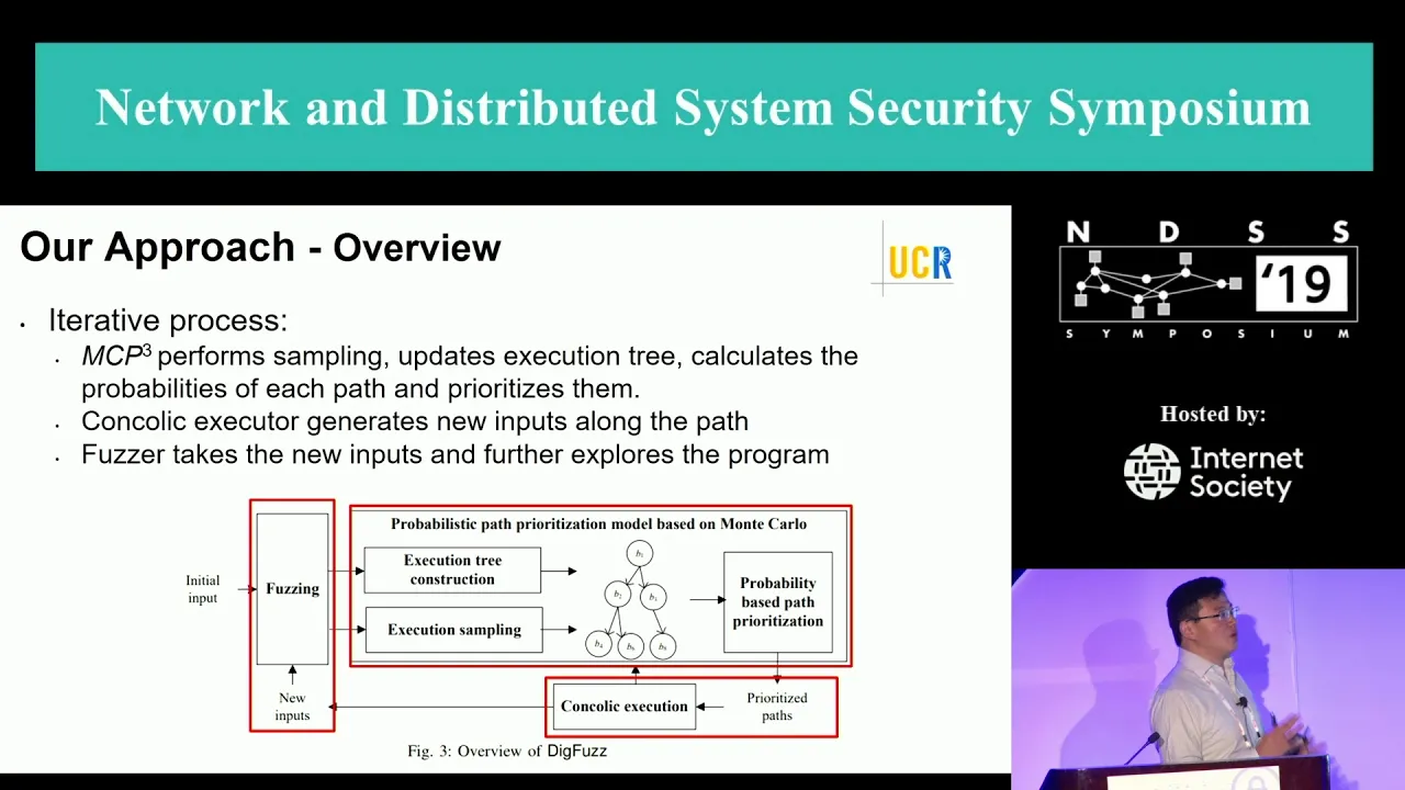
NDSS 2019 Send Hardest Problems My Way: Probabilistic Path Prioritization for Hybrid Fuzzing
NDSSSymposium
496 views•2019-04-02

12:48
Computer Science
How realistic is Cities: Skylines?
CityBeautiful
159K views•2019-02-14
46:39
Computer Science
GUIs & TUIs: Choosing a User Interface for Your Python Project | Real Python Podcast
realpython
2K views•2025-04-04

25:15
Computer Science
The OSI Model - Explained by Example
hnasr
225K views•2019-05-12
1:10:47
Computer Science
Cloud Computing - Introduction
elithecomputerguy
98K views•2019-10-07
2:24
Computer Science
From Traveler's Dilemma to Dynamic Routing | Demystifying Networking
IITBombayJuly
5K views•2019-08-04
Trending

13:38
Law
WOW! Judge TURNS THE TABLES on Trump in His OWN $10B LAWSUIT!!!
MeidasTouch
197K views•2026-07-23

13:25
Business
Playstation NO DISC/NO BUY Fight Is Over...
DavidJaffeGames
4K views•2026-07-23

22:40
Business
Steam and Xbox Just Dropped The Hammer On PlayStation
OhNoItsAlexx
9K views•2026-07-23

16:52
Anthropology
Americans Confused in Australia for 17 Minutes Straight
IWrocker
17K views•2026-07-23