This work elegantly formalizes the leap from individual stochastic spikes to collective neural dynamics using rigorous point process theory. It is a masterclass in transforming biological complexity into a mathematically tractable narrative of network behavior.
Install our extension to search inside any video instantly.
Celebrating 13 Years of Researchat NeuroMat: day 1
Added:Um we are all here to celebrate uh uh this RIC research innovation and simulation center for neuromatics RIC neuromat or sep neuromatic Portuguese uh which is due to finish next month and uh we open this this celebration this special workshop uh a closing workshop of turat now with this welcome session. So the audio speakers will be Roberto Mandes first representing the Institute of Mathematics and Statistics which is hosting this uh this event then with professor professor Luis Mun remotely who speak on behalf of ap research foundation which is the founder of this uh and the main supporter of of the the supporter of this center and then professor Dubafa who is the director of the center will fin give the final speech of this welcome ceremony and then at 9:10 Brazilian time we'll have the first scientific talk by who is in France so let's uh uh oh this initial ceremony will be in Portuguese as agreed so yeah we apologize for that but so the talk will be in Portuguese for speaking Portuguese and then the rest will be in English okay so you can Start.
This is also contra.
Florence.
in particular.
Fore in particular.
Um, uh, Wikipedia is important.
I imagine that importance.
super important.
Science, technology, engineering and math.
form in STEM.
Foreomist astronomy.
Nunes.
against Professor G.
Extraordinary project.
So my perspective my convers political Forever journalist.
Contra.
Fore!
Foreign! Foreign!
Phoenix.
Foreign speech. Foreign speech. Foreign speech.
project.
So Clark Hello, Roberto.
in particular workshops.
I don't know.
Fore principal.
Foreiasm.
How many% defense Flores, Robert Foreign speech. Foreign speech. Foreign speech.
Compliments.
This is for for Wavelets. for I spoke. focusolog.
Clarington.
Bingo.
Fore importance.
participants group.
Fore!
Foreign! Foreign!
Journalism.
It is Institutes United States.
for significant.
My importil.
Antonio workshop.
Fore!
Foreign! Foreign!
So let's go back to English. And according to our schedule, we have uh we start at 9:10. So we still have 10 minutes, 12 minutes to go. So there'll be a short break because we have to respect time. You know, we're very punctual here in Brazil. So we respect time and uh so we'll start at 9:10 punctually with Okay. So you have 12 minutes to rest.
Okay.
All right. All right.
All right.
Right.
Okay, thank you very much uh to for the presence uh in this uh closing workshop of the neuromat project. So we are going to begin now with with a with a thematic session about stoastic neuronal networks and it's very nice to see here many friends that we did during all these years of the of the project and to see them uh um uh talking to us uh about the developments uh they did in this in these years. So our first speaker is Evalerv from Eulp technique in France. She's a a long uh time friend of us and he collab she collaborated a lot and she participated in in all the activities of the neuromat project since the the beginning and working uh jointly with with Antonio for many years. So Eva, it's a pleasure to introduce you you to introduce you in this uh session and she's going to uh talk about uh the Mes maybe you can you can talk your title.
Okay. Thank you very much Eva.
>> Thank you Florencia. I don't see you anymore because I put it full screen. So do you see my slides? I guess. Yes.
>> Yes. Yes. We we can see this.
>> So I decided for this title. So I will read it.
13 years of modeling spiking neurons with stoastic point processes having memory of variable length. And I chose this title because in 2007 when I first met Antonio, he gave a talk in one of the French probability uh conferences and he started with this which is actually the title of a movie which he liked very much and then after that he was speaking about uh chains having memory of valuable length which is one of the research themes that he was working on at that time. So it is to remember this this event when I first met him and when we started discussing.
Um so Antonio Bi and Claudia have asked me to give an overview talk and so I will try to give you an overview of what I think what we did partly on on these stoastic spiking lumen models since the last 13 years that we have been working on that in neuromat. So in my talk I will discuss these point process models for big systems of spiking neurons. I will recall you most of you know because you have already seen a lot of talks by us about this that we will model them as point processes with memory of variable length.
And so I will give the the the big part of the talk is an overview of some of the research activities that we had in neuromat and then I will finish with some open research directions. And of course most of what I'm going to talk about I have learned it from Antonio which you see here. This was the petri master and and from Christopher and it all somehow started exactly 13 years ago when we wrote the first paper with Antonio which is called a system models to to model spiking new. Um so I will try in my talk to to convince you that these point process models are good models to uh to model the neurons that we can use them to explain collective limit behaviors like oscillations and neuro field equations and also to deal with longtime behavior and with memory.
Uh and this is some advertising but I will come to back to that later. As you all know, we also wrote a a nice book with Antonio and Kristoff and a lot of things about these models are written in there actually and in in an rather accessible way.
>> Okay. So the data we are interested we are seeing now um in a Google tab maybe you click something uh >> what do you see?
Oh, it's here.
>> Ah, it's >> um >> sorry. Sorry, we are not seeing your slides anymore. No. Okay, it's okay. So, sorry, you can continue.
>> So, what do you see only? Do you see now the overview thing and with the photo of Antonio and of Kristoff?
>> What? What?
>> Yes, we are. Yes.
>> Okay. So >> I I don't hear you but okay.
>> Yes, we we are seeing your slides now but are not in full screen maybe uh may I don't know if uh before >> that's strange.
>> No it's smaller now maybe you can click them in presentation mode or something like this. Now >> I did it in presentation mode. I can try it. We are not seeing the the slides.
>> Yeah, because I stopped it.
>> Okay.
>> Now you see the slides but they are small.
>> Yeah, this is but in the application maybe you can put presentation mode in the application in the PDF reader.
>> Yeah, that's what I did before. That's why I didn't see you. So this is full screen for me.
>> Okay. Okay. It's okay. It's okay. Like this.
>> Yeah.
>> Okay. Thank you. Sorry for >> no I I should have come. I apologize but it was it was um not really possible. So overview of the talk. So should I talk about all these? No. Okay. I I I start here. So do you see the raster plot of Kristoff here on the slide?
>> Yeah.
>> Yeah. Okay. So we are interested in these spike trains. So here you have an example that I got from Kristoff where we see uh the the subsequent spiking times of three neurons over time. So the time is downstairs and we have neuron one, two and three. Uh these data Kristoff got them after spike sorting.
You all know that this is difficult and not so evident but anyhow so once you have them we are dealing with these data which are point process data because we just um uh say at which exact time a given neuron has emitted a spike and so in the models that we have um we reduce to points. So we do not take into account any special structure and we do not speak about external transport or other things. So as I said each neuron is represented by the temporal succession of its spiking times and uh which for mathematicians is nothing else than saying that we are dealing with point processes and the ones we use people call them multivariate hawks type processes. So multivariate is because we have tons of neurons. So we have different neurons and so to each neuron is associated its own spiking point process and um I say it's a hawk type process because we have this variable memory length. So some people in neuromod also call it the GL models and um the important features of the model are well that we represent I'm sorry for the highlighting. So we represent each neuron actually by its membrane potential process which accumulates the stimuli which come from its presinoptic neurons.
And then there is spiking which is random actually. It it is at a given rate which means that we have exponential clocks but the the the intensity of the clock depends on the height of the accumulated potential. And when the neuron spikes its potential goes back to zero. And at the same time the other neurons they gain or they lose that depends if it's excitatory or inhibitory some additional amount of potential. And this is the effect of the chemical synapsis.
Okay.
So here is the slide for the mathematicians because I will use this um notation later. So um in the talk or in the remaining minutes that I have um I will um consider systems which are made of n neurons and n will tend to infinity. I call x their associated membrane potential processes. So it's x of the first neuron up to the nth one.
And here is the spiking mechanism. So each neuron spikes with a weight that is a deterministic function f of its potential. Which means that the probability of spiking within the next little time bin of length h given the past and given the potentials of all the other neurons is actually something like a buli random variable. It's the 01 event and you accept it with the probability f of x * h as h has to be small such that this is actually a probability and when it is i at which spikes at a given time then its potential is reset to zero and at the same time all other neurons receive an additional potential value which is the synaptic rate of i on j. So we have an associated structure of an interaction graph and here is a picture of that is one of the pictures that Kristoff made for the for the book where we can actually follow the successive um direct synaptic influences of one neurons on anothers. So if you start with number 26 here, it directly influences neuron 20 42 for example followed by neuron 96 and so on. And you can also look on the smallest loop that we have such that the information which is initially emitted by 26 goes back to to its. Okay, good. So that was about the spiking and in between successive spike we just model the the potential by some deterministic flow to to speak about the leakage. So usually we take some uh exponential loss. So so it follows just um a deterministic exponential decaying uh differential equation. We can take other drift functions that is not not so important. Okay. So this is what people call a stochastic integrate and fire model. So stochastic because um spiking or not is a stochastic event. Integrate because each neurons potential is summing up the influences of the presinaptic neurons and fire because then it fires with a weight depending on the potential and people around the Lausan school around Wolfang gasa also call this an escape weight model.
Okay. So this is the the model. There have been a lot of people working on that. I'm only citing mathematicians here and I will not speak too much about that. So there is on the one hand side the people who use meanfield models of integrate and fire diffusion models.
That means that we take a stochastic differential equation driven by motion to model the the potential membrane the the membrane potential of a neuron.
there are a lot of people uh in southern France that have worked on that and in the work we have done in Euromat we basically work with these point process models and that's what I'm going to speak about of course um in the in the rest of the talk okay so I will resume joint works with all these people I'm not going to um I hope that you see my mouse so you see I put in in blue all the neuromat um researchers with whom I I had the chance to work on this. So there are Antonio, Alini, Gami, Kristoff, Puzza, Dasha uh and Kato and and all these others also.
Okay. So I want in the first part of the talk now of the mathematical part I want to convince you that it is sometimes good to pass from this micro structure description where I describe each neuron each single neuron to a misoscopic description and this is basically because the number of neurons that I called n is just very big and so it is not very uh it's not analytically tractable to describe each one of the n neurons if you have 10 ^ 11 neurons which is just a two big uh stochastic system. And this is one of the reasons that people started to work with meanfield models where instead of describing each single neon we describe statistics of populations of big populations of newing that neurons that all behave the same. And what does that mean that they behave the same? That means well they all have the same way of uh reacting to incoming stimuli which mean that their weight functions are the same and um that the system is basically invariant under rotating under permutating the coordinates.
So that is maybe reasonable in some subsystems of the brain and then we want to pass to some limit. So we want to zoom out and we have to do that if you want to do that we have to do it at a scale such that um each single synaptic interaction which is modeled by the uh synaptic weight tends to zero.
Uh and so this is what we do. So we take a synaptic weight that doesn't depend on the pair of neurons which is involved because they are supposed to be all the same. uh and to get some meaningful limit we have to uh to take a renormalization in one / n where n is the system size. Okay. So each single synaptic interaction weight of a given neuron on all of its partners is given by a fixed constant w divided by n and n will tend to infinity.
So together with Anna de Mazi Antonio uh Presi in the follow paper of the one that I cited before we showed actually that in this case we have convergence to a limit equation which call which people call machinoff type equation and where we get an stochastic differential equation for the evolution over time of each neurons potential which is of this kind. The only thing that you I I'm not going to explain it. The only thing is the red term here uh which tells us that the joint action of the synaptic um transmissions of all the neurons on a fixed one. So we isolate a fixed single neon and we just ask the question what is the inference of the whole system on this uh neon doing and in the limit this becomes a drift. So in the limit we keep this w here and is multiplied by the expected mean spiking weight at the given time. So we have the expectation of the spiking weight of any neuron because they are all the same at time t.
And this is why people call this a nonlinear process because the evolution depends on the law of the process. So for people in mathematics that not so evident to deal with these kinds of equations. Okay. So this is the limit equation. So as n gets big each neuron's potential is described by this limit uh equation and we have weights of convergence which is uh something which is classical is one over square root of the system size and usually this convergence works only on finite times which means if you observe the spiking trains the spike trains of the system during some finite time interval this approximation will be valid while it will not be valid up to time infinity.
Okay, these are simulations by Catmo.
So, um it's the pure hawk case. So, if I say pure hawk, that just means that we do not put the reset. Okay, so it's the same model, but the potential is not reset to zero. And you see the the convergence to the mean fit limit on it.
So on this simulation here, we have we see the trajectories of the potentials of 10 neurons and the system size is 20.
Here we also have 10 neurons but the system size is 200 and for 5,000 neurons we have you see that there is a deterministic limit actually okay and we can prove it okay so now I just wanted to give you some overview of of works that we have been doing around these idea of mean field limits so we have big systems of neurons we have some limit system and then you can ask the question what does the limit system tell you about the finite system of neurons And from example, we have been able to prove that the limit system can help us explaining the appearance or the emergence of um collective rhythmic behavior.
And this is something we did some time ago with Susanna Ditlson. I started that when I was visiting her with Antonio. Uh she has also been participating in a lot of neuromat events. So we we looked on the mean feed limits of of these models.
They were structured in several populations. Here it is two populations.
The one is excitatory on the other and the other is inhibitory on the first one. And uh what you see on the figure is um a simulation of the limit intensity and we also see the finite system intend intensities that somehow fluctuate around these limit intensities. So in green I don't know if you see the colors you see that we have limit intensities which have a rhythmic periodic behavior and in dark it is the finite systems approximations and I wanted to stress that these oscillations is not something that we put in the system it really emerges in the limit um or there's a typo just by the interactions between all these neurons and we also added delay in the transmission of the spikes.
So this is one possible um result we had. I wanted also to to mention a paper that we wrote together when Alini and Gami uh were in Paris on the posttock position and we started working with Julian Shuvalier. Maybe I have to be quick because it's already 9:30. But we succeeded to prove that our microscopic uh neuron spiking model under certain um conditions converges to um to the neural field equation which is a very classical equation in in theoretical neuroscience which had been introduced by Amari Wilson and Cohen in the 70s who proposed this equation um to have a deterministic description of neuron activity which is specially um structured actually. So we took our our model but the neurons were attached to positions and the interactions in between neurons that are close to to the same positions do only depend on these positions. Okay, we this is called a um multi-ype propagation of chaos and we were able to prove really uh wigglelessly the convergence to the mean field uh to the to the limit neural field equation. So maybe I just show you the simulations that Julian did at that time. So um well you also see the convergence actually. So downstairs it is the time and upstairs it is a part a slice of the brain. So it's one dimensional here. It's just to be able to to do the pictures. So what you see over time is how the activity evolves.
So red means there is a high spiking activity. Spiking whites and blue means there's nothing. And so you see how this activity evolves spatially over time.
And this is for 100 neurons. For thousand neurons you see already that well there is something very regular which is uh which is popping up. And uh and this is the neuro field mean limit if you want and this is for 5,000 neurons is almost the same. Okay.
So I prepared a slide where we had the equation but because time is warning I will skip this um because I wanted also to mention this paper here. So for the moment I have only been working in in models where the the plus the synaptic weights were fixed. It's w divided by n or it was something depending on on the space divided by n. And um it's very easy in our model to add plasticity and we did this in a paper together with Antonio Erico and Kristoff um where we studied models um where the strength of the synapsis changes over time and that depends on the calcium concentration actually that we have close to the synapse at a given time. And in that paper which was very nice we observed the phase transition in the long time behavior of the model and this is something we know since quite a long time. So it's purely excitatory model and either if there is no outside uh stimulus either the the model will be silent in the long run or we will have persistence of spiking oops well okay of spiking activity which we interpreted as working memory and we see that on this simulation here where we see that the system which initially starts here is attracted to some state when there is a sustained spiking um activity ity.
So this brings me to the question of longtime behavior. So the the longtime behavior of the finite systems and also of the limit systems. This is related to m stability.
Uh and so I cite one of the early results by Alini and Gami uh which you all know maybe. So they showed that isolated systems of spiking neurons if they are purely excitatory and um that they stop spiking almost surely after a finite time. Which means that for the finite system in this submodel the only invariant measure is the all zero state which is the the silent state which is of course not what what we want.
uh but we can see that as the number of new tends to infinity so as n tends to infinity this zero state is actually not stable. It becomes unstable at least for some values of the parameters and since the the finite system also seems to be attracted to some meter stable state.
Um so I try to see how much time I have. I have five minutes. So um actually we can explain that in the pure hawks model where there is no reset to to zero because in the pure hawks model the limit system uh the membrane potential of each neuron is actually described by an ordinary deterministic differential equation. So x of t which is the deterministic membrane potential is so you see the the leakage at exponential weight and we see um the influence of the synaptic interactions w the synaptic weight times f of x of s so the the current membrane potential value of each neon. So if we wonder what are equilibrium states for the potential and that means also for the intensity of each neuron we just have to solve a fixed point equation.
Okay. And it turns out so if you if you write this fixed point I mean if you trace the graph of f it depends on the shape of f but in some cases when it is concave so this red line here is f which is re normalized by the potential divided by the by the leakage weight um no not the potential the synaptic weight sorry so it's little h it should be w anyhow we see that in some cases if initially we kick out of zero sufficiently fast and we have an attracting second fixed point which is actually the meter stable state. Okay, so this is for the pure hogs for the galvar model is not so easy to prove that we have basically the same the same picture.
Well, so we can't directly apply these arguments to the true causes with uh discontinuities due to the reset jumps, but we did it mathematically uh in the paper together with Pierre Mash who got interested in these kinds of models. And so we were in really able to prove that we have major stability in the true GL model where we have reset.
And so this means that we can argue that at least in this model the system remembers some cognitive tasks which are the initial inputs during a long time and the time duration of this remembering of this memory is asmtoically exponentially distributed and I think there will be a talk by Morgan um later today on this meta stability and there have been a lot of neuromat young researchers who have been working on that and Lut Mila and Miguel have just submitted something to SBA which has been um accepted for the special issue for for Anton.
Okay, I skipped this because time is running but I just wanted to tell you that uh these models have um well people got interested in them and this is a guy from uh from N. He did a thesis with itan tore and roman and he was interested in studying the stability of the invariant measures of the mean field limit of the GL model and and actually it's just to tell you for those who are interested so that that's purely mathematic but it's possible to understand if an invariant measure of the nim lassov equation is stable or not you know that for odes we just have to uh to take the Jacobian of the of the drift in the in the fixed point. Uh and so here's also a derivative that is popping up but it's it's more complicated because it's a nonlinear model but people got interested in it.
So there's a lot of research activity that is going on.
Ah so for example right now with the contier and vanmoods we are working on on these kinds of questions for a short-term depression model which is still in the GL meanfield uh framework and we are really able to to calculate the these criteria that assess for the stability and to prove that in some some cases we have sustained oscillations.
Okay, sorry I have to it's very hot in in Paris. So, so far I was only speaking about um the models and that we use the model to understand dynamics. Of course, we can also go in the opposite direction and ask what can we learn about the process from data. You observe that I didn't speak about that. I hope that Gami will speak about that. But it is of course a very interesting research um direction and I wanted just to show you this slide where I give um where I mention some uh statistical results that have been been achieved in in this class of models. So we have the estimation of the underlying interaction graph.
There is this um this work by uh Emilio, Antonio, Janapo and Mao who who really exploit the fact that we have reset to to estimate the interactions and I guess that Gani will speak about his work with Julia. Uh and also right now we we finished a revision together with Alini and Kadmu and Dasha where we estimated the spiking weight of of of a neuron system in a nonparametric way.
Okay. So I have to stop I think because in Brazil people are very punctual. So um I just wanted to close on a on a bunch of open research directions. Some of them are already people started to work on that. So concerning the longtime behavior of the limit system and of the finite one there are a lot of open questions that remain. They are also related to the question of meta stability. Can we achieve that beyond the purely excitatory case? Can we do it in models with several populations or with a spatial structure? Um would be nice to have limit models where the mean field assumption is replaced by a sort of local mean field assumption. So convergence processes on graphs and for the statistical inference there there's a lot of things still to do. I think that's brand new and a very um modern topic. So the the main question is what can we infer about the underlying graph for example if we observe just the point process or parts of the point processes which are involving on it.
Um so I think I have to stop. So what remains after 13 years? So I tried to convince you that we have succeeded to build a rigorous stoastic theory for spiking neuron networks where we have a precise and mathematically rigorous transition from micro to macro which allows us in some cases to explain collective behavior.
Um this convergence from micro to micro opens the road to a lot of statistical inference in some cases and there are a lot of exciting and open questions that are still ahead and so I thank you for your attention. I'm very sorry that I'm not there. This is a photo of one of the workshops that we had at the EASP trimester. And so I really wanted to thank No Romat for these uh well wonderful years. And special thanks to Claudia, Antonio, and Kristoff. Thank you.
Okay. Thank you very much, Eva, for this nice talk. We have uh uh um a little some minutes for uh one or two questions. I I think we have one in from Mao Pichi here in the Mao. Maybe you can speak if you want to ask. I don't know. Or or maybe it's a mistake. I >> maybe you can just read it.
>> Yes. H >> he wanted to congratulate. Thank you, Mar.
>> Okay. Okay. Okay, thank you very much.
Um uh there is some questions for Eva.
Okay, I have a a very very um fast question. Uh do you think in these next steps uh do you think that you can incorporate some uh uh community structures and and your models of uh spiking neurons?
You mean that they are arranged in like in stoastic block models?
>> Maybe but with with time evolution for because uh some some time evolution models with maybe with some behavior uh depending on a community structure of the of the neurons.
>> You for sure you can add this. So um evolution of the synaptic weights depending on in which community you are and things like this. Yes, I'm for sure.
The question is what what is then the the analytical tool that we have to to study them. So what do we want to prove?
>> Okay.
>> Or or to to describe but it's for sure that we can arrange these models in in well spatially or community depending.
Yes.
>> Okay. Okay. Thank you. And other questions?
Okay. So thank you very much Eva. Let's thank again Thank you.
>> Okay. Our next speaker is Gilei Oi O from IMPa now I think or >> almost there. Almost there.
>> Okay.
Nowhere. Yes.
That's why it's not >> now at this moment.
>> Okay.
So, thank you very much, Gilmy. And he's so he's going to talk about rigorous statistical inference for large but partially observed networks of neurons.
Thank you. So maybe you if you can you can speak 35 minutes and then we have some minutes for for questions. Okay.
Thank you.
>> Okay. I will try.
>> So thank you very much Florencia for the introduction. I also before starting I'd like to thank Claia and Antonio Hawk for organizing this u uh closing uh neuromat workshop. Um, and as you can guess from my title, I'm trying I'm trying to to summarize or give some some uh information about the results that I have been uh uh that I have obtained uh with collaboration with colleagues in neuromat related to the statistical inference of a network of neurons. Okay.
So just to be sure that everybody is on the same page let let me try to u define or to state the problem at the very high level. So what is this problem of that we are interested in. So we have data which comes from a spike trains. So we observe the activity of a certain number of neurons. So in this picture here is 13. And then for each neuron we observe a sequence of moments at which uh we we have a spike and here as you can see so here's the time on the um x axis and we uh basically are considering a discrete time version of the data in which we discretize the time in very small bean sizes and um for each bean we assign a symbol one if we see a spike and a zero or the rise. So the black squares here represents a a presence of a spike. Okay. So we are given this data and what uh we want to do at the end of the day is to for each uh is to obtain like is to uh is to come up with a statistical procedure to that outputs a graph where the vertices of this graph corresponds to the recorded neurons and the edges of this graph represent a certain type of interaction between pairs of vertices or neurons.
Um, and of course I mean at sometimes you might not necessarily be interested on this graph itself. You you you might want to understand just some features of this graph. For example, how um what is the density of connections uh that we see that we imagine that we have in this graph or perhaps you you want to say among the neurons that you observe which ones are inhibitory and which ones are excitatory for example. So this type of questions that we um um are interested in in in in to understand. Okay.
So I hope that this is more or less clear the problem formulation and then what I want to do next is just to briefly summarize some of the results that we obtained over the years and then I will try to highlight uh perhaps the the last work that I'm um that I I have um have done together with other people that I believe that can can can have something very important for for the future.
Okay. So what I can say in terms of results? So with respect to the the the question of trying to recover the graph itself, I guess the first paper that we have uh uh was together with Alini, Antonio and Eva. So in 2019 where basically we have we consider a very general um model description for the spike trains. So that's why I'm calling this parametric. Uh we can discuss this later if you want. Um and then uh basically what our result um our results uh say is that we can for for really estimate the existence or not of an edge uh correctly as long as the interactions uh so perhaps something that I forgot that's very important sorry let me go back here um so of course I mean I said that we have a certain number of news uh whose activity was recorded But one difficulty of this problem is as is indicated here in the picture is that there are several other neurons whose activity we don't observe and of course this should be uh should be taken into account in the analysis because otherwise this can be uh can lead to um some spirious um spirious uh interactions and we need to take this into account in the problem.
Okay. So um so I was saying uh in this uh paper from 2019 we correctly we are able to correctly estimate the existence or non-existence of the interactions as long as uh the interactions from uh the unobserved neurons are sufficiently weak. We have a very precise way of saying this. And more importantly, I I think one important u uh uh one important uh point important issue that we want to understand is the relation between the size of the observed network and the size of the number of time points that we have in our data.
which is the relation between these two parameters in uh that allow us to correctly estimate the interactions and uh I mean very in very informally I think our results say that as long t is much larger than an exponential um exponential uh is much larger than exponential of the number of recorded neurons. our method I mean is consist cons consistently estimate the interactions. So this this says that essentially if time is uh extremely big we can really recover the the the the the existence or non-existence of the interactions and if this is not true and then we we don't know how to do it at least with this very general model and then to deal with this fact um we tried I tried with um Patrica Hen so this is she's also a senior researcher and neuromat member. Uh we we try to um use some tools known tools from highdimensional statistics which somehow called this convex regularization methods um to to to to attack this problem of the estimating the graph. And basically here um the idea is that we come up someone can give us a set of functions to approximate the probability of having observing a spike for a given year I given the past history.
Um so we are given the set of functions to approximate this transition probability u through a linear combinations of these pre fixed functions and um and then um the the problem is that which is the the best uh linear combination in the sense that which is the best linear combination which is the the linear combination which is the closest to this transition probability and uh And then once you answer this question, you can really relate the problem of finding this best linear combination to the graph uh to the the estimation of the graph itself. Okay.
And then basically our result says says that okay you might have some dictionaries some some some functions um that you use which really gives you the best approximation. So this is somehow sometimes called the oracle provided that t. So here again the number of time points has to be much larger than the the log of the number of functions that you choose and in particular the point here in the particular there is no there is no um dependence on the size of the network.
So this uh uh indicates that in some cases this me method really allow us to consider very large uh network of neurons which can be something very um interested in pract practice.
uh but the point is that this is this property holds just for um I mean this property doesn't hold in general and uh if you want to uh be um to consider much more complex uh uh dictionaries you ended up again with a condition of this of the type t has to be much larger than the exponential of the number of the recorded neurons times a log term which depends on the the the size of the the number of functions that you use. And again it seems that you are stuck u in the situation where of where you can only consider u networks of a very small size.
Um and then I mean this this really lead us um to the question of uh can we really escape this curse of dimensionality? Can we do something about this? And to better understand um how to to deal with this fact. So I decided with uh with um my colleagues to analyze much simpler uh spike train models and um and I would say that for this uh for this much simpler spike train model I uh the focus for the time being has not been on estimating the graph of interactions but rather we we have focused on estimating futures of this grass of this graph As I said at the beginning, for example, like the density of connections or if I can discriminate for example which neurons are excitatory and which neurons are inhibitory. Okay. And uh in particular so in in this in this framework in this direction uh we recently together with Julia Valier and um Eva we we published a paper where for this very simple toy model that I'm going to present in a minute we are able to estimate the density of connections and we prove that this can be done for example if t is much larger than the square root of n.
something which is much much much um a much weaker condition than the the condition for estimating the graph. And I should mention here that uh this capital n here corresponds to uh the number of total uh neurons in the network whereas in my previous slide this little one here corresponds really to the number of recorded recorded neurons. So this means in particular that for the time being we are forgetting or not considering the fact that we have partial observations. Okay.
So this is something that for this model we uh we are still not there yet. Okay.
And what I want to do in the remaining uh of my talk, so in this essentially 15 or 30 minutes, I want to highlight u recent results that I obtained with Julio uh on on this problem of discrimination between excitatory inhibitory neurons and in particular I'm going to present the the this time model that we have been working on. Okay, so that's the plan for the rest of the talk.
So what is the model? Uh so the model for for defining the model first we we say okay we don't know exactly how the network looks look like how the network uh looks like. So we are going to consider the simplest uh possible model for describing a network where the vertices of this network are partitioned in two sets. The sets of excitatory neurons. So this is the P++ and the set of inhibitor news which is this P minus.
Okay. Um and this set here is just a notation for the set of uh the first n integers which corresponds in my notation to the set of all neurons.
Okay.
So we have the partition of the vertices of the graph and then for each pair of neurons we consider a Bernoli random variable with parameter P.
um they all all they are all independent and if this random variable B I J is equal to one means that there is an edge directed edge from neuron J to I. So there is a direction here which is important and in the model also there is this parameter lambda which uh somehow plays the the the synaptic weight that Eva was mentioning in uh her her talk.
But here we assume that is uh very is a very homogeneous network. So, so um to to to I mean and we quadify every I mean all these elements in a in a graph that I'm denoting here by theta and the entry I J of this graph is just uh 1 minus lambda divided by n times the existence of an edge from j to i. If this neuron J is excitatory whereas if the neuroj is inhibitory it's essentially the same except that we have we we put a value minus okay so this is the graph that we consider in our model and then the second thing in the model is like conditionally on this graph we have a dynamics for the spike trains.
So here we have um xt here is the configuration of all these spikes at a given time bin and we assume that conditionally on the graph we have a mark of model uh which is stationary. So this means that to describe the state of the system at time t, we just need to keep track of the information of the previous state.
And we assume uh moreover that given the state of the system at time t minus one.
So the configuration of all the spikes at time t minus one, all the coordinates at time t are going to be independent.
and which one uh and and the coordinate the i coordinate will spike with a probability which is is denoted by this pi of theta. So depends on the graph depends on the neuron and of course depends on the previous configuration and we consider a very particular form for this transition which is as you can see here in the on the screen. So there is this parameter mu here which plays the row of the baseline parameter and then on the other part here we have two sums. So the first term sum here just says that for a neuron I it look it looks at its neighbors and uh make an average of this the the number of spikes of the neighbors which are excitatory. So this is the first term and in the second term we have something which is kind of the opposite um uh in the sense that um so this is again an average if you want and then we are doing an average effect over the uh neighbors of I which are inhibitory and the point here just to stress that which is important here to interpreted this as inhibi inhibition is that whenever a neuron J which is inhibitor spikes this value the value of x jt t minus one is one so this is zero so really this this this this really um uh decreases the probability of observing a spike for i in the next time and the just to have a I mean just to be sure that we have really a probability distribution no matter the resation of the graph no matter the configuration that you observe this the parameters mu and lambda they are constrained in in such a way but this is just to be sure that we have uh always a well- definfined model okay and so for this model the question that we wanted to to understand uh is okay I give you the the spike trains of uh t um I give you the spike trains of this n neurons and I really want to know which neurons are excitatory and which neurons are inhibitory for this And uh throughout our analysis we assume that we don't have any information from the parameter mu lambda nor the graph.
So this is are not observed and however we assume that the population of the excitatory neurons is proportional to the number of total neurons in the network. So this is n times r plus. Similarly for the neur inhibitor neurons. So the size of the inhibitor neurons is n times r minus.
And um this this parameters they they are both positive and sum to one. But the values of r plus and r minus are not none. Okay. So basically we we we um are not assuming very much on the model parameters.
And to solve this problem we have a very simple solution which is the following I try to explain here. So the u the solution is as follows. So I we are given this data. We compute the average of the spikes for all the neurons. So this is representing this n hat. And then we compute um an average an average of how the state of the system at time t is correlated to the say to the to the the state of the system at time t plus one. Okay. So this is um uh exactly precisely the meaning of this uh uh what we call here one leg empirical conver matrix. Once you do that, you define a vector that we called here sigma egg which basically for each coordinate for each column of this matrix sigma you sum over all the ross uh of this matrix you obtain a number and so this these numbers define this vector sigma egg. Once you do that, you just apply some some um cluster clustering algorithm. We we in our results basically we we focused on the case of a K means clustering al algorithm with K equals 2 because we have two communities. So uh we we we apply the k means with k equals 2 and then we really so and then after doing that we we we the communities one of the communities we we call this p plus and the another the other p minus. Okay. And you can really show that for this metric here. So for a given estimated partition if we if we define this MR of this estimated partition as just the proportion of mclassification we can prove that in fact with high probability the mclassification is smaller than this quantity here. So this this expression which depends on the size of the network and the number of time points.
And uh the point here of this result is saying that rather than trying to uh to rigorously understand what it says is that this method is really um u have uh the the mclassification going to zero as long as this term here. So this term here which means that n divided by t essentially has to be uh very small provided this condition that t is much larger than n. We can prove that with high probability such a simple method works for this model. Right? And moreover we we can prove that in fact uh this condition here. So this condition here t has to be much larger than n is um indeed necessary. We cannot avoid this in this type of problem. And when you combine these two results we we we the conclusion is that uh essentially uh our method is the best we can do for this for this model. Okay. And I mean I just need to want to emphasize that in our results in fact we need that t has to be larger than n times a log factor of t but usually people in statistics they uh they tend to neglect these log terms and um that's why I was saying here that t has to be much larger than n up to log factors and uh we can prove that in fact um this cannot be essentially improved. Okay.
And then just a few remarks. I mean there is another notion that I'm sure that Florencia for example knows that there are you you you may ask yourself you can really not only control the proportion of mclassification which is already something important in practice but also to control the probability of recovering exactly the graph. For this same model, for the same model and a method, we can prove that if t is much larger than n square uh a model with some log factors, we can also uh have exact recovery and our theory in fact I mean allows uh many other possible clustering methods like a hierarchical method or what we call mean and threshold. uh we also have results for spectral method which might be useful for other more general models than ours. So that's why we decided also to study spectral methods. Um and uh yeah so that's that's just a remarks that I had in mind and I don't know if I have much how much time I still have.
>> You have um two minutes.
>> Two minutes. Yeah. So yeah. So in in So the point is okay so we have this theory that says that if we focus for example in the problem of detecting the communities basically we need that the time uh the number of time observation is just larger than the size of the network not an exponential number uh in the size of the network so it's something much weaker much much much weaker and so we have uh theoretical results simulation results that I will deep here and then I just want to emphasize what is the key result behind all this um all this machinery that we developed which I think at the end of the day uh help us to understand the problem of estimating the graph itself.
Okay. Um so this is what we call here this uh I called here key is structure result um and and try to explain this um short shortly but still uh precisely so imagine that I fix the graph. So I fix the graph and then I have the dynamics of our markoff chain. So what quantity that is all be I mean is behind of all uh our results is the covariance it's how the activity of a neuron J at a given time let's say zero because the process is stationary maybe I forgot to mention that how the activity of a given neuron at time um the neuroj at time zero is correlated to the activity of a given neuron I at time one. So and so this is a is something that condition in a graph I can compute this thing but if the graph is random so this quantity here is going to be random as well.
Okay.
Um and so I denote here sigma 1 just to to to is the matrix where I collect all these conditionally coarance um coariances.
And so this is one hand. On the other hand, we have this matrix A here where the entry J is given essentially by the graph. So here I have if uh I take a column which is in P plus the the entry IIG is just the the the graph itself divided by N. And if J is inhibitory, I have the graph again itself divided by N with a minus sign.
So essentially in terms of the the in terms of using the language from the community detection. So this A would be the adjacency matrix adjacency matrix essentially.
And what we can prove in fact is that when I again this matrix sigma one is random because the the environment is not fixed. Uh uh this is something random. And what we can prove is in fact that this matrix sigma one can be decomposed in a sum of three matrices where the first matrix here is proportional to the adjacency matrix. So the constant C1 and the constant C2 here that you see on the screen they are uh explicitly given in terms of the model parameters. So we so that's not very important but we have a very precise um expression for for those constants. So the first time here is proportional to the adjacency matrix. Here we have a bay a bias matrix in the sense that here jn is just a matrix with all entries equal to one. So this is something uh which is a bias term and then plus a error matrix which we can prove that um uniformly for all the entries this is smaller than uh something like square root of log n / n cube. Um and this is important because you see in both matrices here the C1 C2 JN they they they scale as one / N.
Okay. So this is something also important. So this is scales as one overn. This is some some feature which is uh known from the the the the literature of meanfield models. And the error here is something uh which is much smaller than this. Okay. So that's that's important this expression here what is important is that it's much smaller than 1 / n. Okay. And so this is saying that in fact this matrix here this coariance conditioning coariance matrix is very related to the adjacency matrix which is related to the graph itself.
So this is saying that if we are able in fact of getting rid of uh this bias term which there are some general I mean procedures to do that in fact just by studying this coariancy matrix we might be able to estimate the whole graph in fact and the point is uh that estimating this coarian matrix is much faster than I mean you can do this uh for a much smaller um uh sample sizes and in particular this would lead to a condition much weaker than t has to be smaller expon exponential larger than uh the size of the network that's my whole point and in fact uh we are exploring this with uh several people in particular with um um Patricia Henob and um and also with another another um another work within Beru from Impa and Gili Hayes which is a assistant professor in the federal in the federal university in Italoy and um so this leads us to to to the to the my last slide in fact so for this simple model we we wanted to understand a question which was not uh directly linked to the graph estimation itself.
uh but then at the end of the day the tool that we used in fact allow us to relate uh the the the some structural property of the model to the graph uh to the to this graph of interaction and we are we are um think of exploring this this this new uh this new result to to improve our previous results that's the message that I want to to to to say and there are several pos possible generaliz ganizations for for for for this work and of course uh the model is still very simple and progressively we want to uh I mean make the model more complex so that we can go back ideally to a very general model and still uh be able to estimate the graph with a rather much much much weaker conditions. So uh I'm sorry maybe I pass my time and uh I stop here. Thank you very much.
Hey, thank you Gileian for this nice talk. Uh, no, I I think you begin a little later, so it's okay. Uh, some questions no.
Okay. Uh, we have a command. Very nice results from Maro. So, yeah. Yeah, >> I just want to say something. I apologize mu for forgetting for not mentioning your work with medium which is also related to this and it's in within the neuromat uh program but yeah I apologize because this is also something very important for the for for this problem.
very nice talk. Thank you. I have uh just a question related with the if you have any results related with the fraction of inhibited inhibitory and exitary networks. I I believe that this when this fraction is like one half you need like the most data to have a good estimation.
Can you make any comment about that?
>> Yeah. Yeah. So in fact I mean in the paper so if you look at the paper we uh we I mean I should say Julia did the simulations um and so again the model is very simple and the par parameter values were exactly this low I have um p is equal to 0.5 I mean in fact all the parameters are are equal to 0.5 except mu which is 0 255 just be to to be sure that mu is uh and lambda are constrained as they should be and so and for this particular um choice uh I think the network is balanced so we have 50% of excitatory and 50% of inhibitory our method which would corresponds to this so in this table here we have different values for n and t so you can see them here And what we plot here are the the the percentages of the mean classification rate. So it means that we simulate several times 100 times and for each time we apply our procedure and then we compute how many u mclassified vertices we have. And you see for our um for those virus here our our um mclassification rate is around 2%.
And uh in fact there is another procedure which we call this uh threshold procedure which performs performs best for this parameter values.
And basically um I try to explain here just very shortly. The idea of this of this uh mean threshold procedure is like you take this vector gamma vector gamma hat compute the mean value and do your classification with respect to this mean value. All the coordinates which are above this mean you put as P plus and all the others you put as P minus. And so since there is this special symmetry in the problem this very simple even simpler than K means algorithm uh performs um better.
But then when you change uh for example when you change the the proportion of excitatory uh if for example if you increase this as will be uh more um close to the reality our our our result our method works much better.
In fact and uh of course I mean there is something that is very important that I forgot uh for the theory was very important that the P here which controls the density of connections of your graph is keep is is kept fixed and then of course one natural question is if you can uh allow this to change to scale with n to have sparser graphs and so this is uh one of the things that uh is we are uh currently work working with uh Patrica Henobu and we hope soon have some some um some some some results about that.
>> Okay, thank you very much.
>> Okay, let's thank Gile again.
Okay, thank you Gileiam. And now we have a a little break for a coffee. And ah yeah, sorry.
Ah um Arur, can you put the the the messages in the or because I I'm not seeing here.
No, no, in the the messages here.
I think previous commands or >> no he added some some comments recently.
So um he said oh no it's I I don't know.
>> Yeah I think it was a kind of question for me. Uh >> yes. Yeah.
>> I said we didn't use the fact that a neuron is either exitary or inhibi inhibitory. Yeah, >> of course. Okay.
>> Yeah. I tried to answer to him, but yes, Moto is just um for >> Yeah, just not a question, just a comment. Okay.
>> Okay.
>> Thank you.
>> Okay. So, thank you very much. We we will do a a little break now and we'll return in 15 minutes. Okay. Thank you.
Great.
Fore! Foreign! Foreign!
All right.
Okay, let's uh continue with the with our session now. H our next speaker is Morgan Andre from EMUSPI and he's going to talk about about the pathways approach to metastability and its application to GL models. So thank you very much.
Uh okay so thank you very much for for the invitation for this talk.
uh which uh is in time because uh I when uh I was asked to give a talk to kind of summarize one of the line of research of neuromat. I was just finishing a paper with with cardmo about metastability in GL models and so this is what I will be talking about and trying to to summarize all the the different results we obtain in the different version of the car to shop model.
But uh so what is uh metastability in general? So it designates a tendency of a system to dwell for a long time near an an apparently stable equilibrium before a rare fluctuation nucleates in on a comparatively short time scale a transition toward another equilibrium.
So in short, you could say that metastability is something any system that that has a behavior which is kind of between uh stability and instability.
Um so it's a notion that has a a pretty long history starting in mostly in chemistry and physics and then was observed and studed in many different areas such as economy, electronics and specifically neuroscience that become it has become an important topic because neuroscientists believe that the brain is metastable for some reason and um well I do not really have time to enter to the details of of why is that and I will focus most more on the on the mathematical part but uh so from the theoretical point of view like in math and and theoretical physics there were different approaches that I've been developed to to study metastability and um uh you know dynamical system and stocastic pro and so on. So one of them one of the first one is the evolution of ensembles.
There is a pricewise approach uh potential theoretic approach and spectral approach and many others and I will I will focus uh on the on the pwise approach.
Um which is which um so there is a there is a kind of a seminal paper.
Ah, okay. Okay. So, sorry for shall I stop and wait a bit or stop and wait a bit.
Um yeah so I'm going to focus on the password approach which basically um was invented after the evolution of symbol. So I will just quickly speak about this first evolution of ensembles approach which comes from a paper of the 70s by pen and leovitz.
Basically the idea is that so you have some uh evolutions that it can be it can be a deterministic evolution like dynamical system uh with possibly random initial state or it can be a stcastic process typically like interacting partic mian interacting particle system and uh so let's say you have some so s here the blue part is the state the general state of the of the of the process or the dynamical system in R is some candidate for for metastable region.
And in this evolution of ensemble, the way they characterize u metastability is uh suppose you have some some um probability mu invariant for the system and you take the the conditional uh uh version of mu on the um metastable region R.
And then you consider the probability uh along time PT that the system gets out of this uh region R.
Um so you can imagine for example if it's a dynamical system so you choose the initial state with respect to this m me mu r and uh then the system just evolve and you can at some time t it can be either still inside r or outside r and you you you what you're going to consider is the evolution of this uh polarity distribution over time t and one of the uh um fundamental property of metasable system. So it's not the only one that's maybe the most important one in the the three uh uh characteristic properties that you gave is that um if you so you would like the proity uh uh to to become um bigger and bigger uh as as you can change some parameter of the model. So typically the number of particle maybe the temperature and so on. And what they do is that they look at the at the derivative of this of this uh probability of being outside air at time t. And you can prove that uh the the the maximum value for for this is actually at the the origin at time zero. And uh so you look at the derivative at time zero and the the requisite that you want for for the system to be me stable is that lambda can be uh taken. And so lambda is this the notation that you take for this derivative at at zero. It can be taken as small as you want. Um as you uh changing the parameter of interest. So you you might think typically the number of particle even if it was not the actual parameter that was considered in this original paper.
uh which is a way to capture the fact that uh uh this this ex the the escape from the the region R uh um can be very very long uh uh for for for relevant cho choice for the parameters.
Uh and so then there was another paper in the in the 80s uh by uh Cassandro Garves, Olivier and Paris uh called metastable behavior of a stoastic dynamics a password approach which was kind of um an alternative approach to this evolution of a symbol by pen and lab and they did this uh this uh observation that one of the problems that you have with This approach uh uh is is single trajectories dwell for a long time to the equilibrium is you have you have difficulty uh distinguishing between two different very different situation uh if you're looking only at the polarity distribution of or the probability of getting being outside the meta at time t right so you're just looking at the pollution of a polarity measure over time uh you you it's very hard to distinguish between the the situation which is actually metable where you have single trajectories which dwell for a long time near absolute equilibrium before making a sharp transition to the true equilibrium.
And another situation which is completely uh unrelated to metastability and the the every single trajectory will uh uh go outside R but in a very slow and smooth uh way with where we don't have this sharp uh uh you know pod stationary phase for some time and then a sharp like tuneling uh to the outside of the metabol region uh which is basically you can see it that way uh um um with this with this picture here. So typically you you would look at some energy profile like your free energy in the meta table with the left one where the so you can imagine that the ball is kind of getting randomly uh um on the left and on the right and you can see that in the situation on the left it will uh stay stay in this uh in this valley on the left for some time but at some point because of some random fluctuation it will eventually get here and then cross the the the energy hill and and go down the actual actuallyable states while uh if you're not looking at at every so it's called pass wise because you're looking at individual trajectories and estimating the probabilities and if you're not doing that you could not see the difference between this situation and and this situation here where you basically have just a very very uh uh flat slope And you can take you can take it as flat as you want if you changing the parameter in some in some direction and it will just very slowly go to the equilibrium. But this is not metable at all. You just have one uh um stable equilibrium and the the the system just goes there um in a straightforward way.
So as a result of this observation they propose the pass wise approach to meta stability which is uh so the imagine you have a micro system of end particles and uh you have two uh fundamental properties for characterized metastable systems which is first you look at the extinction time on some micros opic time scale beta n and it has to be to converge. So it's always an asmtotic property when n goes to infinity and you expect you expect if it's metastable you expect that this extinction time the time it take to get out of the metastable region will be exponentially distributed um which and this is because of the memorylessness of of of uh exponential distribution right and so this kind of cap already capture a bit of the of the pathwise uh perspective Because I mean you can uh um differently from this uh perspective where you look at the polity distribution over time t uh um and eating time you can see it as some kind of functional over trajectory that gives you some information and it captures some of the information on complete trajectories and the fact that it's memoryless it means that you you cannot so if you if you know that the system is alive at up to some time t give no give you no no information about what's going to happen in the near future.
And then you have the second property.
It's called termalization uh which can be expressed in this complicated mathematical way. Basically it means that you have another uh kind of smaller messoscopic time scale on which if you look at basically uh any kind of special temporal statistic on the system uh over over this methoscopic time scale you'll see that for big n it's close to some kind of constant value and so the system is just wondering uh um you nearby some fixed equilibrium.
uh this is before before the escape from the meta stability region.
So and what about galva model? So let me just define in a general way what I mean by galva model or gl models. So basically I mean on the on the most high level viewpoint GL models are interacting pawn processes. So we can imagine that you have a family of pawn processes on the timeline.
So positive reals and uh and and the the point of this of this point processes are the spikes of the system and like almost any other point process it's it's I mean the formal way to define it is that way so you look at this so any small interval infinal interval uh you you have one spike at some rate lambda it t where i is for non i uh and you have two spike for in a very small interval with priority zero basically and um and that's all. And the difference with typical like a simple person process this kind of thing is that we're looking at the conditional property with respect to the to the filtration of the system. So basically this lambda it the rate of the spiking is something random that depends on the past of the process right uh and it depends in a nonlinear linear way. So you have the mebr potential and the the spiking rates is basically a function of this typically nonlinear function of this mbon potential that I call f here and the moment potential is just a value for the for any given neuron as a given neon potential mbon potential that depends on the on the fation of the system and uh okay and so what's what's really matter is how you define actually this moment potential But how how it will integrate the spikes from the in the previous activity of the system. And so I will define this in the next slide.
But a last thing is you have so you have also um synaptic weight giving you uh for any two neurons the strength of the connection. It can be either positive or negative meaning that the the connection can be either exidatory or inhibitory.
Uh and that's all. And under very weak condition you can show that the system is well defined.
uh but so this moment potential how is it defined? So you have different uh version I call it I call it GL model with S because actually you have you can see you can define various different uh variant of the of this of this system that are uh more or less equivalent but uh use different mathematical tools to to to model uh uh the dynamical system. So maybe in in particular one of the difference is how you will model leakage.
And so maybe the most uh straightforward and uh you know bio biologically realistic uh is um is continuous leakage. What I call continuous leakage meaning that so the leakage is just the fact that the moment potential tends to decrease continuously over time. And you will model that just by some uh function here G uh that will tell you how how fast the neuron basically forgets uh its past.
Um and and here you have the spike. So any anytime a neuron spike it it transmits some some extensation or inhibition towards the other neurons. So given neuron is integrating the spikes of the all the other neurons. just uh kind of getting some input uh positive or negative input as each spike of the other neon in the system and whenever it uh it uh it does the neuron itself spikes it will reset itself right so it some value for the mobile potential it just get to zero which is included in the model with this lit which is the formal way of representing the viable lance memory of the of the neuron Um and one particularly interesting um um instantiation of this model is when you take uh GT as an exponential function with some rate alpha negative exponential uh because uh first of all it's quite natural choice from the biological point point of view because this is the same kind of things that were used in more classical like leaf uh uh you know lapic model and and so on but also it makes the system marking right. So what what we have here when you look at the system of potential. So you have the evolution over time for all the neurons you have a PDMP. So um um what is this uh u um deterministic peacewise deterministic microp process uh meaning that you have a jump but in between jumps you have this exponential decay. So which is deterministic and this is a pace deterministic part and you can write uh so the dynamic of this whole system in a more compact way using just you know classical theory of microp processes using the infinity infinity generator so how much time do I have more five okay and uh so another way to to two way of modeling leakage which are a It's more a bit simpler mathematically speaking. It's a bit less u um um realistic biologically but it makes the model more tractable is our total leakage and unitary leakage. So total leakage the idea is that you will just model the leaks as another process and at each of these total leaks the system just abruptly lo not the system but the neuron abruptly lose the value of its potential and unitary leage is the same kind of things. We have a also um the pawn processes for the leaks. But instead of losing everything every every me potential the wall value of the membrane potential at any of this of the atom of this pond process we will just lose a unitary amount of of moment potential and so these are three version of of the grav model.
So two reference for the continuous leakage. So there is many more reference actually but these are maybe the two that are more um relevant for the cons the question of metastasability. There is this paper from this paper from Alen Dwart and G O which is not about metastasability but they looked at the at the extinction time the eating time and prove that it was uh almost surely finite in uh in under some weak condition which is necessary to then consider proving metastability and then metastasability was proven in a specific direction of this continuous leakage in a paper from evalar and P Mar uh um in 2022 and u this is not working anymore.
uh total leakage there is well there was a few papers that uh I did uh during my PhD thesis and then during postdoc uh period and uh where you have I would just consider a simple version of a system where you have uh one or kind of binary activation function just basically a simple um uh intering particle systems and uh there is a paper also from from KMO liar uh in the same kind of of of setting meaning total leakage but with a a function that is not a binary but it's an explosive function for the activation function and then there is unitary leakage that was considered by Antonio Marcos in a cment uh where it's not a result about meta stability but it's a result about face transition in is a system that is defined on on a tree homogeneous tree and then a paper by uh is the same paper actually. So this paper here it it did both total leakage and unitary leakage.
But um so what we did with Kadmo writing this review was trying to summarize all but also to to kind of um highlight the common structure of the proofs and how you get to to show a literal conf. So what for the first property of the of the memoryless extension time. Basically, you want to prove that this goes to zero, right?
When when n goes to infinity. So, you're proving that you're losing memory. The the synthetic time is losing memory. And you do that usually by getting some bond on this with two different terms uh one in on on the part of the space which called WN and the other one on the complimentary of the sets. And this is WN is basically uh uh the typical configuration inside the metastable region. And um the the W and comp the complimentary of this is asypical u um um the art atypical uh states uh uh that you expect anyway to to to be unlikely for big N. And so the way you prove that both of these goes to zero is inside W.
So the first term it's always some kind of renovation argument where you use some kind of maximal coupling. So you consider two different system and define them in a way that they will agree um the most possible way the anyway you will they will be the most uh they will agree together as far as possible. let's say and uh and then you can show so here you have usually a difference between uh um the extension time starting from two different places and you can show by this coupling usually this maximal coupling is close to zero and outside W you use some uh proxy of the system so usually you can show that either you take the the meanfield limit of the system or you have a modification of the system which has some invariant measure mu And you use the the the information that you can get and prove with respect to this proxy and its invariant measures to to show that uh uh uh this thing uh goes to zero.
And um yeah, how many times do I have I'm dead already. Okay. So I wanted to to to speak uh a bit more um closely uh um on on one of this on this the paper from from Maria about the continuous leakage but I will have then to to um to skip it because it's been too long.
Um just let me um uh mention that there are there are also many other works on metab that were uh done but in a context a bit different from the setting that I just presented either because it's mostly numerical result because it's not exactly the GL model in the in the in the specific setting that I indicated here or either because metastas is not really studied in the past wise sense uh that I I introduced in the beginning of this presentation but uh yeah and uh yeah okay so here here's a summary of this all these results and um so I wanted to to end up uh talking about some of the of the questions that are still hanging and so just very quickly one of the question is beyond the meanfield or compensating so many times what what you do is uh so you have many uh degrees freedom in the model, right? It can be the activation function, the type of leak and so on. And one of that of that of this um degrees of freedom is the the topology of the interaction graph and and almost all the results that were done, you have a mean field complex setting, meaning that all neurons interacting are interacting with the other neurons basically the same way, which greatly simplify the proof. And so we we're able actually to do the proof in that kind of setting. But if you go out of this kind of setting meaning that you have some special features and the things get messy and the question is how can we under this this type of of cases.
So what about animation also most of the of the result that were obtained were obtained in purely extatory systems. So the question is uh how can we obtain such results with inhibi in inhibitory neurons multi-stability if you have different metastable phases and you can you can just pulling from one metastable phases to the other like continuously and um and yeah so tamilization so this is the second part of metastability that I I I spoke about in the the beginning but most of the of the result just focused on the first part so this It will be nice to have some time to to take care of the other part as well. And the last one is one term. So in this the slide that I just skipped because um because the slides about the result from Mar. So one of the remarkable things that they do is that they prove a general results for obtaining meta stability for kind of in a model independent way like for some kind of general mark of uh process on some uh polish space.
And the question is whether or not we could use this kind of general result to u generically um take care of most of the models without having to do very specific u hypothesis on the on the activation the various degree of freedoms that we have for defining the model and that's very much uh Morgan for this for the talk. Uh some questions.
Okay. Okay. We are running out of time.
So maybe if you have comments or question we can do it in the lunch time.
Uh so now okay now uh it's my my turn.
I'm be I will be brief. Um I first would like to to thank Antonio and Claudia for the organization of this nice workshop. Um as as many of uh Bafa and others uh talk we had many workshop during the the the during the the project and this is this is an activity that that has been recurrent in the in the project and I think it's very nice we we had the opportunity to do many friends during these 13 years. So my goal is to talk a little about past and present developments in the statistical analysis of neural neuronal random networks. It's it's the the title maybe is is too broad but I I'm I will only focus in the works I was involved with h with many um many researchers of the of the project.
So first first of all I would like to dedicate the the the talk to Antonio and Kristoff that unfortunately are not with us. And of course, Antonio was the the person who who who took who created all this and make made this possible and um enable that we could do and participate in many activities and and and did many uh friends in this during these years and Kristoff also was a person that I I didn't have the opportunity to work with him but uh was a very important person uh during all these years of the project.
So only to to talk about to talk a little about the history and and my personal history in this uh project.
This began when this is a photo for my from my defense in 2007 here in this in this not not the same room because it has been renovated but it was the previous one and uh we had here many friends and and people that contributed a lot to the project during the the years. Pablo Ferrari, Ricardo Fryman, um Nancy Garcia, Roberto Fernandez, and of course, Antonio, my supervisor. And so we had a long history working with many people that uh contributed to this project during all these years.
And as I said uh we had many many workshops and activities during this 13 years of neuromat. In particular I I put here h the the workshops that were related to random graphs and random structures in the brain and h statistical analysis of these structures. And so they were very very important for for h the activities of of the project and was something that and Antonio did a lot. He was very good organizing activities and h putting all people together to work in some problems. And I think this was uh one of the points that made the the Neuromat project uh to have such a success that many people mention today in the opening.
So I only put this of course there are other activities in other h other lines but I I put this because it's the more or less the the the the works I I I did during this year and when we from my perspective past development that we did here inside Negroat this was one of the first uh works we did with Claudia Danielle that are here and Andresa Cada that now is a professor in the Federal University of S Carlos and was my PhD student, master and PhD student and at that time um we began to discuss uh about how to analyze uh random graph data built from from EG data in this case from the from the brain and this was very nice we had very nice discussions Antonio was not an author of this work but of course he is in in the behind because he he was the person who put us in contact and and made it possible. So um h we we discussed how to construct this these graphs from the from the brain and how to analyze them statistically. So this one was uh uh the first work we did in 2017 and only to talk a little about it we we had some data that was collected in the laboratory Claudia's laboratory h about an exper about about an with an experiment of people seeing like a movie of a some light point of a of um person uh walking and we have uh we had two experiments. One was a a uh like the point representing a a person that was uh walking and another that was uh a scrambled point. So the idea was to construct some graphs using this DG data. Here we have a pipeline how we constructed the graphs. H uh the the so the data was collected uh during this experiment. The pe the the persons the individuals were uh seeing this this movie and we had two faces in the movie. One the visible facive face where the the the person was walking and another another h part where nothing occurs.
So the the the data was the the EG data was collected during all this time and okay I I I had to cut the the figure because was very large. So here we have the EG signal and then with this signal we did we transformed this in a in a correlation matrix uh between the the signals. So uh once you you transform this signal in a correlated matrix we can in the next step construct a graph of this between the neighbors. So here is a map of the of the EG a map of the EG channels and here are the the edges connected connecting these uh pairs of neurons using as a base the the correlation matrix that's so this was a very simple idea and it's it's very but it's very used in in many experiments and how to construct the graphs and the idea was to see if we can distinguish the the the different experiments and uh the the different phases of the experiment and the the two experiment that we had that was one was the bi biological movement and the other was the the scrambled movement seeing the uh samples of graphs we obtained with this procedure. So in the work we I I'm not going to talk about the details because we don't have time but h in the work we analyzed the the random graphs that h we obtain and we developed a a test of of hypothesis to um distinguish between populations of graphs. Um so here you have a like a consensus graph for the biological motion. Here is the the scrambled motion the two experiments the visible phase of the experiment and the uh occlusion phase of the of the experiment. And and we saw uh differences in this uh different scenarios.
So uh This was the the first work we did as I said uh seeing the analyzing graphs for the for biological data for brain data and uh after that uh I begin to work with uh uh communities in in graphs. I have an error in the title sorry random graphs.
So um in in the second I I began to work with uh community models uh in particular stoastic block models that are models uh probabilistic models that emulate uh the communities in the in the graphs. So it's a a gener a generative model that uh shows a structures of communities and this began to be a a thing that uh was somehow uh there are some people interested in this type of of models in the in the neuro science community. For example, this is a figure for from this uh work weighted stoastic block models of the human conneto across the lifespan. So in this in this work uh the authors uh show different adjacency matrix and the corresponding block model that shows this structure.
So you can have different community structures in your in your graph and this translate it translates into uh a specific block model. So this is was a a work showing the use of these models for neural network. In my case, we be I begin to to work with statistical properties and probabilistic and statistical properties of this uh model and only some commands why why the the stoastic blow model is interesting for for neuroscience.
Okay, so these I think are commands in this previous uh paper that I cited.
They say that the human brain can be described as a complex network of anatomical connections between distinct areas known as the human conneto. The fundamental characteristics of the connetos organization can be revealed using the tools of network science and graph theory. And of particular interest is the community structure of the network where communities are conceptualized as densely interconnected and sparsely h densely interconnected and sparsely interconnected. Okay, it's a intra maybe densely interconnected and sparsely interconnected. I think maybe is the correct phrase. It's a it's an arrow. So that is the communities are characterized for no that are connected with the with the same inside the same community and that has not too many connections with the with the other communities. But as the talk in in H as Gilei talk today we can have other also other structures as the the heatory neurons and exitatory neurons that also show h community structure in the in the network. So in this in the inside this model we have some mathematical statistical and computational challenges that uh for example to mention some of the problems I I have addressed in these years uh in general you have this generated model that is the stochastic blog model but you don't observe the the communities in your model you only observe the the the the the graph and when you observe the graph you cannot see anything. You cannot uh see the the structure because the the notes are uh totally scrambled and you cannot detect erh only seeing the the image the the community structure. So the problem is not easy and you can have different problems. For example, one is to estimate the communities to this means to to to uh cluster the nodes in the communities.
Another problem is uh estimate the number of communities with some statistical approaches. This is known as model selection. Also to propose a study efficient algorithm for the community detection and model selection problems because computationally these are difficult task and uh also study or propose more complex models related to the stoastic block model for example state space models random dot product models and so forth. So h so one example was the the model you hear me presented today that is a a kind of a stoastic block model for a particular model for neuro biological data. So this uh this um study of the stoastic block model gives some works in the in the last years some with some works with Andrea about the the estimation of the number of communities in this model or in in a related model that is called degree corrected stoastic block model and more recently a work uh showing optimal recovery of the of the communities with maximum likelihood Erh okay but uh as we are running out of time I I will not talk specifically of these works I only give the the references and if if someone is interested we can talk a little more about about them and talking about future developments. So I talk about the past the more or less the present or recent past and and and recent recent development and now some future development.
Now we have this uh national institute of science and technology in stoastic modeling and complexity that's was uh approved by CNPQ in the in the last year and was the idea was uh to continue these lines of of neuromat now neuromat is is coming to the end uh next next month and And we uh so uh we submitted this uh project to CNPQ uh to continue and to to continue the the development of uh statistical probability uh uh and computer science uh developments and applications in in neurobiology and health. trying to do a framework framework to have uh to enable the the lines of the neuromat to continue h in this project. So this project is coordinated coordinated by Lis Renato Fanches here from EM and Nancy Garcia from Uni Campi.
And in particular uh one of our of the of the activities that were we are planning is a workshop in August about mathematics. How ma can mathematics contribute to artificial intelligence.
So one of the maybe this is one of the future development we want to um to uh put energy in the future in the next years as a continuation of of neuromat.
Um so uh the the how can okay how we can what we can do from mathematic mathematics to uh the development of artificial intelligence for neuroscience or or or health. So uh this is our contribution to the next years of of these lines. So I would like to to thank you for the attention and we now have uh the other another online session. So I I will finish here. Thank you very much.
Um yes. So let's move to the next activity of this morning session uh which is a tribute to Kristoff.
Um, hello. Hello.
Can you hear me?
You hear me? Yes, you can't hear me.
Can you hear me, Eva?
We can't hear you. Yes. Not yet. But it will come.
>> Yes. Now, now it's fine. Thank you.
Thank you very much. So um let's start again. So the next activity will be a tribute to Kristoff Puzza.
Um thank you for your presence and uh we are very touched by the um willing of our colleagues and people from Neuromat to this activity here today.
So we would start uh uh with Kristoff's contribution to neuroscience by Alan Marty.
>> Yes.
>> Uh do you hear me?
>> Yes.
>> Uh can I show uh my screen?
>> You can share your picture, your slides if you want. Yes.
>> Yes. I'd like to Uh, I'm trying.
>> Hello.
Can't share with me.
>> Okay.
>> Go here. Go here.
Uh >> just wait.
>> Okay.
>> Maybe I should just talk.
>> You cannot see my screen, right?
>> No, I should.
>> No, we can.
>> Uh you can you see me?
>> Yes.
So I'll start. Uh so all of you or most of you know the uh recent uh kind of graying Kristoff Puzza. I would like to present the uh Kristoff Buzza of the end of the 1990s when he was aged uh 25 years something like this. So I met him around that time. He was a brilliant physics student in Paris and I had my lab also in Paris at the time. And um later he wanted to start a PhD in uh experimental neuroscience which is what I did. At the time my lab had moved to Germany. So he came to Germany and uh more or less in in 1995 he joined the the lab and he started his PhD thesis with with us. So he had a background in physics but he picked up biology almost immediately and he started to produce um beautiful results groundbreaking results that ended uh up in a series of very uh beautiful papers. I can't go into details because of lack of time but uh this was really a remarkable achievement. He studied the elementary signals rising at the single synapses in the rat brain and uh he in particular followed this as a function of of age during early development which is something that was unknown at the time and also he discovered a new uh a new signal which was um which was in the pressaptic neuron but it was a retrograde signal. it was a noto receptor current which was totally novel and which is uh still intriguing at at at this time. So uh all of these achievements are are quite remarkable.
Uh but also due to his personality he engaged himself in the group activity.
He uh developed analysis uh procedures software that we have still uh using now. Are you hearing me?
>> No, nobody's here.
>> Yes. Yes. Yes, we hear you.
>> Okay. Because I can't I I have I have absolutely no feedback. So uh analysis that we we are still using now and um also more surprisingly perhaps he introduced anatomy procedures that were not used in the group at the time and that he uh picked up somehow and introduced for the benefit of the entire group. Also the most amazing thing at the time for me was that he very rapidly acquired a cleareyed view of the uh literature in that field of of of science. Uh and he pointed out to me uh cases of over interpretation of the uh then um prevailing um uh theories about the the mode of transmission of synapses and of possible errors in the publications of prominent laboratories in the field at the time. So uh from conversations with Kristoff at the time uh that helped to orient my own research uh actually up to up to the present time. Uh and that of course you would not expect at all from a beginning uh graduate student. Um so when I followed a little bit later the um the career of of Kristoff, what was evident was that he was not so interested in promoting his own career. Uh much more interested in uh improving the quality of the science around him. For instance, he tried very hard to uh to improve uh the rigor of our approach to statistics of us experimentalists and that was moderately successful I should say. uh on the other end of the spectrum he also worked a lot I think uh to convince um theoreticians to be a little bit less naive about the complexity of biological data. Um more recently few years ago we organized a a course in uh Colombia in Cali Colombia 19 2019 course uh that was a twoe course and uh Kristoff was uh was uh in charge of informatics. We were in charge of uh more the experimental part. So uh quite recently one of the students of the course told me that she uh she really loved the uh the the the lectures by Kristoff that previous to that she thought that informatics was boring but that uh Kristoff's lecture changed this completely and she also told me that uh after the end of the course so this was co years uh Kristoff continued with webinars and the students of the course followed these webinars and they kept active and they kept uh in contact with Kristoff for many months and this was very important for them because remember that this was the the time of uh of uh the pandemics. So I have to stop here. I think uh in short the uh the achievements of Kristoff at the time of his thesis work are really remarkable and uh they are still um influencing our science right now. Um more importantly I think what is remarkable is is his unique personality which is made of sheer generosity instead of of following uh the the the implementation of his career and and building a a small uh scientific empire which he could have done. He was more interested in uh sharing his knowledge with the people surrounding him. So I'd like to stop at this stage. Thank you for attention.
Do you hear me?
We hear you but I don't hear the >> Yes. Uh there were some hand claps.
Thank you very much. Uh >> okay that doesn't okay for a very nice >> Is there any question or maybe we we have to wait until the end of the session for questions.
>> Patricia is asking a question I think.
No, sorry. I was trying to clap but I messed up with the signs. But thank you so much.
Thank you.
Any other comment or question?
>> Thank you very much again. So >> this is difficult because Kristoff was such a unique director but I think it will be more apparent from the uh the the next uh interventions as well. Thank you for organizing this. Thank you Alan Marty. Thank you very much. Eva, do you want to comment on it? Vera, sorry. Vera raise her hand. Thank you Vera for being here with us today.
>> Uh thank you so much. Thank you very much. That was a very touching uh talk about Chris. So um uh thank you all. Hi, I would like to thank the Neuromat community to um think of Kristoff today and to um organize this session which is very moving. I'm with my son Pascal and um Kristoff and I uh met during his thesis um with Alan and um this is full of beautiful memories. Thank you all so much and it was a pleasure. I had the occasion to be once with Kristoff um at the neuromat in Sao Paulo and it was a great pleasure for those who remember me um to share time with you. Thank you very much >> so much Vera. Now Eva lob is going to talk a little bit about Kristoff's contributions to neuromatics. Right.
Thank you Eva.
>> Yeah I try to to share my screen.
Um just a second.
I have to pull put it full screen now.
Um you all see my my slides.
>> Yes.
>> Okay. So I start with the photo. Of course this is so this is a photo that we took when Dasha showed us um the forest of Fonten Blue. That was right after the trimester that we organized in in Paris two three years ago I think with uh Antonio Claudia Kristoff and me and you see on the photo you see Kristoff uh Alim Dasha and myself. So I I try to to remember when we dis started discussing and when I first met Kristoff but actually I don't know but um I can tell you the following. So um we have not that many uh publications together but they are very important for me. So we wrote one paper together. I will speak about that later. And then most importantly we we wrote this book together with Antonio on um probabilistic spiking urinary nets.
>> I I can hear >> okay and so I will speak about um about the book first. So actually Christo's contribution to the book was really essential. um Antonio and myself we we had some book project since a long time.
Uh but it was only when we started discussing with him that that this project uh started to to to to be alive and that that we slowly understood where we wanted to go and what we wanted to write. And uh so for example he shared his uh knowledge which is very deep about point processes and and their appearance in theoretical neuroscience with us. He brought to our attention the the articles by Willinger and um and so I wanted just to advise you to read at least two very beautiful chapters of our book which have been written by by Kristoff. The first one is um well uh is uh the appendix number B. So the book is um is written in two parts. The first part which is a a general one and then the second one where we have complimentary material. So it is um this appendix on the two landmark article articles where one of the two landmarks is byer. So he discusses this article and he makes the link with the general linearized uh model. So I just copied here I can't show anything with my mouse but uh one extract of what he was writing. So Kristoff is um insisting on something which was important for him.
So he writes a generic software which was called GIM was already available at that point. So that was in the 80s and this software was thoroughly tested uh to fit the GLM model to data and uh and he discussed that brillinga discussed this um this software in in the paper. So Kristoff writes that makes him not only the most important contributor to spike trainer analysis but also a pioneer of reproducible research and you know that this was one of of the important things in in his research um interests.
Okay. So that this was one thing I wanted to point out. So this is in the book and I also wanted really to invite you if you have not already done so to read uh the chapter one that he wrote in the book uh a neurohysiology primer for mathematicians. So it's written for half of us here in the in the audience. uh he explains everything you should know about neurons starting from the membrane potential and the action potent potentials and not ending with the questions is is there a global reset when when there is a spike or not? So do we need to add reset or can we stick to to the classical hawks model that we discussed earlier in today's session.
Okay. And so in what follows I just wanted to show a couple of slides because uh every well almost everything that I know about u is Kristoff who explained me with a lot of patients uh and in particular he explained me why we should bother with spike trains why it is important to have a stoastic uh element when describing them and so why stoastic intensity based models for them are a good modeling choice. So this I I already showed it before. So this is one of the pictures Kristoff used to show. Uh after having sorted the the spikes of the different neurons, you get the spike trains. So these uh samples of um point processes over time.
And uh why should we study spike trains and not the exact uh evolution of the membrane potential of a neuron? Because uh and this is the answer by Kristoff. I completely copied it of his slides. The the key working hypothesis in neuroscience is that it is the time when the neuron spike and not the waveform of the spikes which are the the main information carriers between brain regions. And this is the reason why it is a good idea to to study spike trains and to develop models who will be able to predict the probability of occurrences of spikes in the future.
without uh too much considering the biohysical spike generation mechanisms behind. So we we don't use hskin huxley models or these things. We really use these um hawks type models and this is I would say one of the main aums that was underlying a lot of neuromat work around the the the GL model.
Um this is another slide by Kristoff where we he tried where he answered to the question why we have to to add a strong stochastic element when speaking about spikes of neurons. Um so for example we have the stoastic opening and closing of ion channels which can lead to fluctuating spike trains and then there are also fluctuations in the synaptic transmission which are observed in successive responses of the same synapse to to the same stimulus because the number of synaptic vesicles which are released day by one activation to the next. uh there are states where the ion channels they can switch from closed to open states and so so on and so it is clear that we need some um stoastic element to model this. This brings me this is why I was speaking about that.
So I wanted to rapidly also speak about our GSP paper which was about short-term uh plasticity and how synapses work.
That was the common work with Antonio Erico and Kristoff on a system of interacting neurons with a short-term synaptic facilitation.
Um, so maybe I skipped this. So basically here we considered synapses that evolve over time at time scales which are comparable to the spiking activity of the network and we these variations are due to the residual calcium whose concentration is changing over time. And at the point where we wrote the paper, there were a lot of papers in the neuroscience community that had been written about uh short-term potentiation, but most of them were purely numerical studies. Um so for example, there are famous works by Mark Sodics, Kistla, Fanhman, Zolza.
But I think that the work we did um with Christo was uh I mean we we posted proposed a single model mathematical model but we could do precise and rigorous um proofs in these models and in particular we were um able to identify short-term memory with the tendency of the system to keep track of an initial stimulus and um well that's written here. This is what Antonio used to say about it. these short-time memory. We can interpret that by the capacity of the the system to stay in certain regions of the state space which are actually untypical uh and which we can interpret as um uh as a feature of this memory. The technical tool we used is the passage to mean field limit. So to a large population limit together with precise error bounds and then in the limit we have a twodimensional dynamical system um which we can actually then study. So we did this here these these are simulations by Christo. So it's two-dimensional because we have the membrane potential and we have also the the calcium uh concentration and we showed that in the limit OD um I have to stop also I I'm I'm almost done. So we showed that the limit OD process is actually equilibrium points that are not present in the finite system and of course that should be related to met stability. this is something he he was interested in and and we we see this as an indicator of short-term memory.
So I wanted just to say this here the the last phrase. So I think this work reflects the way he worked. So we try to capture biological phenomena which are interesting within a simple model uh by doing still a rigorous mathematical analysis.
So yeah, that's all I This is a photo that Vera took of us at some point. So uh so of course I I I learned a lot of him. I um we had thousands of discussions. We um we organized a tree master together. But uh above all he was he was a a good and a very dear friend.
So I I will stop like this.
Thank you. I don't see anything.
very much ever. Now I would like to move to Borgan Andre who is going to talk about Kristoff as a mentor and supervisor please. Yes, sure.
Yeah. So I I didn't prepare any slide or anything.
Um well because I didn't want to to share just objective information you know in scientific achievement soon and I'm the other one did that very well. So I will just u um give um tell you three short and highly subjective stories about Kristoff and my personal relationship with Kristoff.
So the first one is um Kristoff as an advisor. So when I was still a master student in Gob in France, I needed at some point writing a master thesis right to complete my degree and I contacted a professor in Paris which I knew for my graduation and this person was not Kristoff. was um because I didn't know Kristoff at that time but it was one of his colleagues Barin and uh he agreed to be my my adviser so I went to university parat at that time when the name changed so much during the last year that I I don't know how it's called today but to discuss the subject of my future master thesis and um and so I met Kristoff at that moment because he was uh he was present at this meeting because he was the quarter of the paper which was to serve as a starting point of my master and so shortly after I started working on it and I would uh frequently go knock on Aar's door to ask question and try to cry for and so on and he was quite uh busy and after some time I think he got a bit annoyed by my insistent questions and um politely asked me to figure it out by myself. Um so then what I did figure out is that I could um maybe knock on Christoff's door and I quickly realized that I would always welcome my um my stupid question and take the time to think about it and help me out and this is basically how Christophan end up becoming my my main advisor.
But um most importantly this highlight one of the many qualities of Kristoff which was his natural kindness and the fact that he would always consider you regardless of who you were distinguished colleague or wonder master student or really just any complete stranger and it strike me retrospectively that that if it was not for his kindness I would maybe not being here talking to you and I've done something maybe.
So this was the first one, Kristoff an adviser. So now the second story is about Kristoff as a colleague.
Um so as years passed he went from being my adviser to being basically my colleague and as such uh Kristoff was kind of the Rosetta Stone of Neuromat because um he was a very com combination of you know substantial um biological and and physical knowledge and also solid mathematical background.
And so it was a keystone allowing all the various people of of Neurumat with very different backgrounds uh to be able to communicate with each other to understand each others and he prevented that the most mathematically minded of us drift too far from reality into esoteric abstractions.
He was also a very truthful person and he will always um tell his honest opinion in the most straightforward manner and that I personally like very much about him even though I guess it may seem a bit rude sometimes to some people.
And the third story is Kristoff as a friend. So I just realized that it's been almost 12 12 years now that I knew him. And over the years um we've become not only colleagues but also friends and in the last few years uh it had become kind of a tradition for me to visit him and his family everywhere in Strasburg.
So I would go there and spend a few weeks in January or February usually at the Puzza family's home Rodu Canal uh to work on whatever we were doing at that time and um so during the week we will go to the lab at Sor University and at night we will have will have dinner together with Vera his younger son Pascal and sometimes his daughter Sophie and then have a long discussion on on science cinema and politics to sometime late at And uh sometime it felt like we did not agree on anything but it never really um matter at all because we were it was clear that we agreed on all the rest.
And the last time I saw him was during my visit in last February.
And um so given the type of conscious he had I knew it was possible if not likely that this will be the last time I would see him. And uh being the statistician that he was, he was certainly well aware of the odds. But uh we just did the usual thing and went to university and pretended that it was just you know business as usual.
And this may highlight the third quality of Kristoff which is bulletproof, calm and modesty.
So yeah, that's all for this reason and many other I will miss him very much and yeah thank you.
Thank you very much. Merc's also thanking.
Okay. So now uh I'll talk a little bit about Kristoff Puzza and Neuromat. In fact, I made a very short text and it's called Kristoff Puzza Antonio Galves and Neuromat.
Uh, as far as I know, Antonio Gaus and Kristoff Puzza first met in 2013 at the workshop mathematics and neuroscience, a dialogue held in Uted and coordinated by Roberto Fernandez.
I clearly remember GI claiming that this very shy and brilliant researcher had exactly the profile neuromat envisioned a combination of a mathematician and a neuroscience experimentalist.
We later discovered that Kristoff had several other unique features that he generously shared with Neuromat including rigorous scientific thinking and a strong commitment to open science in March 2014. Antonio Galves writes to Kristoff. Dear Kristoff, Roberto Fernandez just told me about the excellent presentation of your research in in your habilitation thesis. In particular, he mentioned the analogy you drew between a statistical mode model selection process and the concept of free energy in physics.
I reviewed your publications list and I think Hobbert was referring to the statistical methods you developed for sorting action potentials.
But before I continue, let me tell you why I'm bringing out I myself have been trying for some times to un to understand the concept of the quality price ratio which has been used in neuroscience notably by spawn as a candidate for the principle of conneto reorganization after a stroke or other type of injury.
I'm wondering whether this has anything to do with the principle of free energy minimization.
I am trying to place this within a framework of statistical model selection and I've been asking Heru for a while how to link the principle of free energy minimization with a model selection principle like the maximum penalized likelihood.
It was through this repeated question that he told me about your articles. How do you see the relationship between the principle of free energy minimization and the model selection principle?
Best regards, Antonio PS. and congratulations on your abilitations on your abilitation to drive to Dijer after I think it's this is very typical of of a conversation between Antonio trying to convince Kristoff to to join the Romat team at that time. So after this email exchange in early 2014, Antonio and Kristoff met again in July that year at a seminar organized in Cophagen by Susan Dit lives. At this seminar, Anton invited Kristoff to join Aromat and visit S. Paulo. This first visit took place in September 2014 and marked the beginning of a long series of Kristoff's very productive but sometimes also turbulent voyages to S. Paulo including challenges such as air strikes and credit card losses and also a very very nice visit of Vera and Kristoff at some point to S Paulo and to which was very cheerful for everybody here reflecting on this initial visit Jean Pesonski recently said Kristoff's visit to Brazil during the early days of S Pisn Romat in 2014 offered one of our first opportunities to adopt a broader approach to scientific dissemination.
It was a complicated period. The dissemination coordinator, Professor Hamburg, was absent and we lacked the strategic vision. Working with Kristoff consolidated or even initiated several key actions. Film production, Wikipedia editing, uploading to Wikipdia Commons, press outreach on works in development, hybrid events, music production, open science reflection, and organizing scientific conceptualization.
With Kristoff, we produced Neuromat first internal video which won an award.
Kristoff embraced all these ideas with enthusiasm even though they were entirely new to all of us. From 2015 onward, Kristoff actively participated in the preparation and curation and served as a conference chair in almost the Neuromat seminars, international workshops, courses and several Lascon.
His detailed, beautifully prepared, very cultivated and clever presentations were a through gift to all who had the chance to watch them. These pearls were often hidden behind his shyness and sometimes excessive scientific rigor.
During the coid9 pandemic, he attended all the online seminars organized by neuromat. He also actively worked on the preparation and production of the parkare meeting held in Paris in 2023 as mentioned by Eva. After Antonio Gaus passed away in September to 2023, he continued supporting Neuromat in several ways together with eval by completing their beautiful work by orienting and exchanging with young researchers as Morgan told us today and by supporting our more recent scientific activities. Kristoff Puzza became one of the pillars of the neuromat project for which we are deeply in depth. Today we mourn this incredibly unique person.
Thank you very much.
So the neuromat team prepared some uh presentation. Yes, the video this was done by Juan Peshanski and Taiis with some pictures of of the the period of Kristoff during this all these activities and we just collected them together in the I don't know.
Think was a king.
A big challenge is how we can build models that are incl. inclusively stoastic and still simple enough so that mathematicians can manipulate them, obtain themselers can simulate them efficiently.
Well, thank you all for your presence.
If uh the microphone is open for those who want to say some words, please be free.
Dr. Marty ever somebody in the audience.
>> I would like to repeat what I think is the uh defining characteristic of Kristoff was his uh generosity.
Please go ahead.
Claudia, can you hear me?
Yes, we can.
>> Uh, thank you so much, Claudia, for setting up this beautiful meeting and for your beautiful memory of Kristoff.
That was uh very touching and very nice.
I thank you all for this um tribute to Kristoff uh to his work to his personality and um I very much appreciate all the work and all the the pleasure also he has been taking in working with you. It was always a major project for him to go to Brazil and to enjoy the collaborations and um thank you to all of you. Thank you so much.
>> Thank you very much. Thank you.
So we we um would like to end the session by thanking everybody for their presence and their words. Thank you.
Okay, thank you very much Claudia and all of you for this nice tribute to Kristoff. Uh so now is uh in our program we have a time for lunch and we return at 2 pm. Okay. Oh, thank you.
H. Uh, let me try something else. Can I call you in a moment?
I'll call you back.
>> No problem. Sure.
Okay, let's see.
What's going on here?
Can you hear me?
>> Yes.
>> Can you see anything? No, not yet.
>> Uh, the sound is a little bit low though.
>> Yeah. Let me first try to see if I can share this window.
>> Great. Now we can see your slides.
>> Can you see it?
>> Yes. There are a little bit behind me.
>> Okay. Can you hear me now also?
>> Okay.
Uh, is everything okay? Um, Claudia.
>> Yes.
>> Okay. So, I wait for your for your command to start.
>> Oh, okay.
Give me just two minutes please because we are just just adjusting. There's >> no rush. How long should it be?
>> Uh can you please keep talking so that we can adjust the the the >> volume?
Yeah. Just um how long uh uh should the talk be?
>> Yes. So you have um 30 minutes.
>> Perfect.
>> Okay.
Yeah. Yeah. Yeah. Yeah. Yeah.
>> Perfect.
Is the sound okay for you? Yes. Okay.
Very well. Let's start then. Right.
>> So, everybody So, can you hear me then?
That's good.
>> Yes. So, let's I'm I'm making a little a small introduction for you, Leo. So, it's a great pleasure to have professor Leonard Coen today with us. Leo Coen is uh has been a frequent partner and collaborator of the Neuromat project since the very beginning and he was he has been member of the international advisory board all this time long. So it's thank you very much again Leo for all your partnership and contributions to the project. Okay. So you can start whenever you want. Thank you.
Thank you. Thank you very much um for everything. Thank you for the uh input that I got over the years in through nomad and it's been very it's been inspiring in a number of ways these interactions and part of those are expressed in one of the uh themes I'm going to be discussing with you. Um it's been uh a pleasure also to integr to interact with all of you over the years and uh and well I'll tell you a little bit about what we have been working uh on our end.
Um the uh interest the general interest in my lab or one general interest in my lab has been the study uh of the um uh neural mechanisms supporting early skill learning or early learning of naturalistic skills which is something that I always I have always seen as potentially uh uh useful.
important in the clinical context in uh with the goal of uh uh allowing patients with brain visions to relearn uh skills that have been lost after they are for example uh strokes.
So as a background, skill learning involves forming new memories that bind discrete actions, for example, single piano cipes into complex spatial temporal sequences like for example a musical refrain or a small song.
Uh when we start learning a skill, there are prominent gains that occur very early on that are followed by near plateau performance levels. And then after uh performance plateaus, there are somewhat smaller additional gains that develop in between practice session across periods of rest.
uh a phenomenon that has been labeled as a consolidation or as offline gains.
Uh a few years ago, I'm going back actually to 2019. Marlene Bonstrom who was a fellow in the lab at the time was interested in trying to understand better uh how does learning develop across periods of practice and rest.
Um and uh she asked healthy subjects to practice a press piano sequence for one three to four over and over again over alternating periods of practice and rest for about 36 practice trials on day one and then people came back on day two to retest that skill.
What she found at the time is that when this uh when people are exposed to this initial practice session, performance uh expressed here in the form of uh tapping speed or key presses per second improves very rapidly over the initial practice trials until performance reaches about 95%. % of maximum and then somewhat the performance plateaus and when people come back on day two for testing you can see that there is a small additional jump here. This phenomenon has been termed as overnight consolidation.
And at the time Marlene was very interested in this initial period of very steep learning which she uh um characterized or defined as early learning until performance reached this near plateau.
What she found at the time in looking at performance improvements across periods of practice and rest was that and she labeled or she defined changes in performance during practice as micro online changes and those in between practice periods as micro offline periods. The micro refers to the fact that uh were periods of practice and rest of only 10 seconds duration.
And what she found uh as a surprising finding at the time was that the total early learning was largely accounted by micro offline performance improvements that develop across rest intervals rather than practice itself than during practice itself.
This is something that was very surprising for that was very surprising for us at the time and that was later uh reproduced in uh primates and in other human experiments extensively.
Um so in this particular experiments uh what happened was that that was published last year uh uh it was found in two different task motor learning and visual spatial learning in these monkeys that performance improvements developed predominantly across these rest intervals rather than during practice itself.
So the summary of that initial work was that early naturalistic skill learning unveiled at least for these challenging tasks unveils predominantly across rest intervals.
Uh we found through a number of other experiments that physical and cognitive fatigue during those small periods did not affect these learning dynamics.
And we also uh um concluded that micro offline gains stabilized over time consistent with a rapid form of consolidation that develop over seconds.
So these findings as I mentioned have been extensively replicated in the literature.
So we next uh uh looked at the kinematic mechanisms that uh cause this phenomenon. And this was done by William Kisler who was a PhD student in a combined uh um PhD program with UCL in London and Sven Bestman.
And what we did, we did this experiment in which uh people learned the task I mentioned and while they were while their performance was videotaped and then we used a number of software um tools that were just published in Current Biology this year, leading us to be able to characterize the develop velopment of combination of digit synergies that allow this learning to occur.
So what you are seeing here in the at CISA are the same 36 practice trials uh when people learn this task I described earlier on and what you're looking in the yaxis is the percentage use of synergies including different number of kresses per synergy from a single digit key press per synergy to much more complex synergies that engage simultaneously four or five different key presses.
And you can see that initially people engage when practicing the task in the first trial predominantly a single key press per synergy like expressed here in the green colors to some extent two key presses too. But as training progressed, you can see a progressive reduction in single digits uh key presses per synergy towards a progressive increase in multi-digit synergies as people get better and better.
Um the next point that was interesting here was that these synergy changes develop predominantly across rest intervals that is um uh micro offline as shown here rather than micro online.
And importantly the magnitude or the um uh magnitude of change in these synergies from single digits to multi-digit synergy predicted the magnitude of learning during rest but not during practice.
So uh what this meant was that high order multi-digit synergies emerge across rest periods of early learning.
They consisted of small rapid and overlapping digit movements that predicted rapid consolidation and raise the clinical question of to which extent or if if we understand which are the synergies that best allow performance of the skill or best allow expert skill. If it is possible both in the context of the clinic as well as in education to train synergies in addition to tasks as if in for example closed loop um neuro feedback protocols.
Imagine a piano player who uh is trained on a particular effective synergy rather than generally on a task or a music student. So this is an interesting hypothesis that we bring up in this paper this year.
Uh we then moved on to or actually we did this before but for the purpose of this story we then looked at the uh possible uh CNS mechanisms that could support this form of uh learning. In other words, how can individual key press action representations bind into a consolidated sequential skill across these rest intervals during which performance improves and uh we posed at the time that neal replay could be one factor. Neura replace the compressed reactivation of neural activity representing sequential motor behavior during rest.
We know in rodents that reactivation during nonrem sleep is linked to skill consolidation.
We also know in humans that fMRI activity in the hypoc campus during these rest periods predict microline gains.
So we thought at the time that it is conceivable that wakeful neural replay during these rest intervals can contribute to rapid consolidation of skill.
uh in this work done by Ethan Bush and Leo Cloudino who's originally actually from Brazil uh the uh we look at MEG activity while uh subjects were learning this task.
So MEG was acquired over 272 channels source localized and parcelated.
We then train decoders on the practice data. First single subject individual SBM decoders and then performance was cross validated in a different data sets in the form of a confusion matrix.
We then uh look uh uh with these uh decoders trained on the practice data at the probability of single key press reactivations during rest data then the probability of sequence replay detection and then uh the data was significance tested.
So following this pipeline uh we look at the MEG activity when subjects were learning this task and this is what we found here in the X-axis. You are looking at different possible replay durations based on animal literature that characterize do different durations of replay events.
Uh in the y-axis you are looking at the number of replays per second occurring during those rest intervals and you are looking at three analysis of three different periods. Pre-training rest before people even practice the task. Post-training rest after practice completely finished and then at rest intervals alternating with the practice periods.
And what we uh found here was first that the replay rates triple during training rest intervals relative to pre and post-training rests.
that the optimal replay duration was about 50 milliseconds when the actual behavior which is the time required to complete the keeper sequence that was being taught was about 1 second.
We also found that looking at the overall replay count, overall subjects and trials and the interre replay intervals that replace did not occur one at a time separated by regular periods of uh without replay, but rather they occur very close to each other at very short interre replay intervals that is they occurred in bursts.
So we concluded that the train skill which is the keeper sequence was compressed about 20 times because the optimal replay duration was 50 milliseconds which is 120th of the 1 second uh duration of the actual behavior. So the train skin was compressed by 20 times and replayed largely in bursts of about 25 replays replay events for each 10 second rest interval.
We then found that approximately 70% of the total variance was in a principal component analysis was explained by a PC1 component that included the sensory motor cortex interrinal cortex hypocampus and precunius.
We also find found that the um difference in replay events per second or the increase in replay events per second was specific for the uh trained sequence but not for untrained sequences.
and importantly that the replay rates correlated with rapid consolidation for the train sequence but not for the control.
Importantly, these results were replicated in invasive studies in humans at least twice uh last year.
And also importantly in the uh in a recent experiment in primates it was found that the uh activity during these rest intervals was very important for these jumps in um h performance.
So the black lines are showing the uh jumps in performance across the yellow periods which are the rest intervals.
The yellow periods are the rest intervals. And but if you apply a form of interfering brain stimulation, in this case it was beta uh alternating current stimulation uh between others during rest. It blocked learning as you can see here. So in other words there was a there is a causal link between this rest activity replay activity during rest and the behavioral offline gains.
So in summary from that work motor practice elicits wakeful compressed neural replay.
is predominantly represented in sensory motor medoral memory regions.
It predicts rapid consolidation of skill.
So this mechanistic work then we were interested in trying to find out if how does this apply uh perhaps in clinical settings and we haven't done much we have not done too much on this front but we try to evaluate this in patients with long COVID in a clinical study William Hayward did this a couple of years ago and he was able to show that patients with long COVID in this blue analy in this blue group were showed a reduced overnight consolidation relative to age match controls.
So uh from that uh work uh we are now studying patients with memory disorders between other uh things and starting to look into stroke patients as well trying to look at the sources the basis of these um perhaps anomalous neural replay in situation ations of different pathologies.
So with this I will I would like to thank and to acknowledge a number of collaborators and the institutions that uh funded this work um in our environment and thank you as well and I wanted to leave perhaps uh a little bit of uh couple of minutes for questions that could come up.
Thank you very much.
>> Thank you very much Leo for this beautiful presentation. So questions.
>> Thank you. Go and uh I'm here.
>> I'm here.
>> Oh, you're out of the camera, but that's all right.
I need you to stage two of >> I can hear you.
>> Okay.
>> Now I see you.
>> Okay.
Uh my question is about do you think if we work with a condition with a mental simulation not with the the actual realization of the motor movements that uh could be interesting to understand how we can think about the way that we make the junctions of each one of the event and the expectation about that >> it's a very interesting question It's a very smart question and it's definitely something that has been in the uh um in my mind but uh but it has not been done and I and to tell you the truth I'm not planning to do it. I think I'm waiting to some extent for uh some pipeline to uh characterize neural replay events from EEG because that will make life much easier for everybody and will allow a much more extensive investigation than what we were able to do in this case with MEG.
uh but conceptually it's a fundamental question that needs to be addressed. I completely agree.
>> Yeah. My other question is about the EG but you you said before. Thank you.
>> Ah yes yes. Uh I can tell you one more piece of information. I know of somebody in Japan who's been uh developing or who has been able to characterize replay on EG. uh he recently shared with us the because we asked the um the methods of the non yet paper of the non-existent paper and we are going to be looking at it but uh uh I'm trying to encourage him to publish a technical contribution to address it because it will allow a much more widespread investigation of this phenomenon than with MG.
>> Okay. And I said because we exactly have this data the the data >> absolutely I'm sure that's why I wanted to bring this up to nomat because uh because uh that data is probably available in many many people's labs uh without knowing how to analyze it and this would be very very important.
>> Thank you.
>> Thank you. Any other question or comments?
Okay. So, let's thank very much Leo for his beautiful talk and let's keep in touch.
>> Thank you. Great seeing you.
>> Thank you very much. See you. Byebye.
>> Ciao.
Our next speaker in this statistician brain session is Alin Di from S. Paul.
Thank you Alen for giving this talk today.
So I would like to start thank you clouds and hockey for the organization of the uh of the workshop and our final event and uh uh clouds and hockey invited me to speak about context three models and how we use them in neuromat in this uh last 13 years. So I will give you a introduction a more or less mathematical introduction about the context tree models and how we use them to do some experimental protocols and then the results uh I will uh leave to cloudy and maybe Marcela will also speak a little bit about this kind of data. Okay.
So we are interested in well let's just uh before well we all believe that actually brain is able to uh identify some uh patterns like if I give you a pattern one two three one two three one two three very quickly uh you realize that this is a pattern this is not a doubt we all believe that this is true and this is really accepted in the neuroscience and even for people which are not from neuroscience right but What we would like to answer and I think Antonio was very uh positive about is the brain is able to figure it out or at least uh understand or at some point or at some uh find it that actually we can realize even more complex kind of uh patterns. what I mean by more complex patterns. This is why I will try to uh um formalize for you today. So what is complex pattern? For us in neuromat at least we believe that a complex pattern is something which is not deterministic.
It's a probabilistic sequence and a very specific a very specific kind of a uh complex pattern or probabilistic sequence which are the ones coming from context tree model and when I say it's very specific it's not very fair actually because almost any kind of stoastic sequence we can uh describe with a context model this is why I will try to convince you today okay so what we want to do is okay We know that brain is able to uh realize deterministic comp deterministic patterns and I will try to convince you at least that we can do this even for uh complex patterns. Okay.
And the four things I have to to define to you is how we will characterize this kind of complex pattern. So for me in this u uh talk uh complex pattern would be characterized by a istocastic stimuli or a stoastic stimuli. So I have x1 x2 xn is stoastic stimuli if you don't know what is a istoastic stimuli is for for you could be a probabilistic sequence.
So I have a sequence and uh I don't know exactly what the next step's going to be but I have a probability a probability that something is is happening at each time. Okay. And uh for each stocastic stimuli I will record some kind of data.
So could be a physiological data or a behavior uh answer. Physiological for us would be for instance electronographic data or any kind of physiological data you can imagine or behavior and like um if the person is in some sense realizing about the complex or not. Okay. So you depend for the second one you depend on uh a answer a directly a active answer of the volunteer. So in case of uh for me in this uh talk I will uh keep two different uh kind of experiments. The the first one is when my stoastic stimuli is given by some um sounds. So I have here some bits x1 x2 xn are different kind of bits. So this is in some sense is a kind of rhythm and then I'm recording here some functional data which is actually electronolographic data. Okay. And the second type of experiment that I can have is when we have for instance a game. So here my stimuli are the kicker.
So the kicker will choose for instance um left, center and right and uh following some stoastic uh sequence or some uh probabilistic sequence and the volunteer is the goalkeeper. So you have to guess where the kicker is is is kicking and then you will choose center, right and left depending on what you are guessing.
Okay. So your answer here the performance is also uh left center and right. Okay. So this could be one zeros and and two 012 012 for instance. We don't need some function here. So I have two different kind of data and two different kind of answers and what I will try to do today is defining this properly. how we define this stoastic sequence and how this answer here relates with this how this y1 yn relates with uh x1 xn okay and then claudia will speak a little bit more about the results so for me I have two kind of stimulas this 21 zero could be strong ws weak wids and silent units or right center and left so this is for the rhythm experiment and this is for the goalkeeper experiment. So for instance if I start with a deterministic sequence given by 211 211 this is the kind of pattern that we are not uh we don't have any kind of down that brain is able to realize right but let's suppose that I take this sequence and then for each one for each symbol one I will uh decide if I keep one with probability 1 minus epsilon or if I will exchange this one by a zero with probability epsilon in some sense for each one here each symbol one here I'm flipping a coin and if this coin is a tail I will keep one otherwise I will replace one for zero okay then this we know that the brain is able to uh realize what is happening but for this one which is probabilistic and stochastic we this is what we want to answer is the brain able to characterize in some sense this uh sequence this is what I'm calling complex pattern here.
Okay. And when I say is the brain able to characterize the first things we have to realize is how we characterize that in order to look at for characteristics right so how I can characterize this sequence this is sequence and the way we do it is usually at least uh one way of doing is through context trace and how we do that so let's suppose that this root here is the present which are calling I'm I'm calling xn n and for this line here I will put all uh possible um events that can happen at time uh n minus one. So the the step before the present could be a two, could be a one and could be a zero. Okay, if the step just before was a two, what would happen? Well, after a two, we know that the way that we construct a sequence, we know that after a two, I can have a one with probability one minus epsilon or I can have a zero with probability epsilon. This is the only two things that can happen and I will never have uh two followed by another two. Okay, so I can summarize that in this line. So each time I have a two as the previous step, the next step will be a zero probability epsilon and a one minus one with probability one minus epsilon with probability 2 will be a one with probability 1 - x. Okay. Okay. So for two it's easy but let's suppose that the the step just before was a one and then I have more or less a problem because I have two different types of ones. For instance, I have the red ones. For a wed one, I have two different events that can happen before. I can have after this one another one and after uh this kind of one, I could have a zero, right? So, I'm taking the ones which are coming after a two. And there is this these two possibilities.
And I have other kinds of ones, the blue ones. For this kind of one I will always have a two with probability one. So basically I have two different cases. I have once which can be uh followed by one or zero with the coin that I eras in one probability epsilon one minus epsilon or I'm in the case where I I don't have choice. I will go to a strong bit just after this is because we construct the structure like that. So in the end what I'm what I'm saying is actually looking at the single symbol one it's not enough. So what I'm saying is type one and type type two of ones or red or blue ones actually is the same that saying that I have to look at two steps in the past. So if I have a two one I know that I can have a zero with probability epsilon and a one with probability 1 minus epsilon. If the last two steps was one one then I don't have a choice. I have to go to the uh symbol two with probability one and so on.
Okay, is it clear to here?
And for the zeros I have also the same kind of problems. I will have uh red zeros and blue zeros. For uh for blue zeros I could have a one or a zero probability one minus maximum maximum.
And for the type red zero I will always have a two with probability one. Okay, so this is the same as say as saying that actually zero by itself is not enough to predict what is going on in step n. So I have to look at two steps on the past and then I will look at 0 0 1 0 0 2 and so on in order to predict what is happening in the present. Okay.
So uh what I'm saying here actually is basically what I just did here was characterize our stoastic sequence through two different things. One thing is this set which is basically telling me uh how I can split all the possible pasts in order to have all the options that I I need and for each one of these these possible paths I'm associating a transition probability. So in the end this set and this family transitions probability are characterizing completely my istoastic sequence. Okay.
And we call this uh the the elements of this set uh context or basically I'm calling context all the leaves of this this tree. Okay. So I will just skip the formal definition because I will not have time. Uh just a small comment this kind of model was introduced by hissen hissing as a universal universal system of data complexion and in the literature you can find also with the main the name of stoastic chain with memory of variable length and variable length markup chains.
Okay. So if you remember the first picture that I present you, you have the volunteer and then you give him some uh stimuli which I just characterize it here as a context model and then you well the picture leaves some uh data right something that we are recording. I just explained to you define it what is the first part. Now I will try to define how we associate this the second part the in and the X.
So how we define this dependence suppose that we are recording our experiment. So uh the brain is recording the stimuli and you have seen the stimuli up to time XK.
How do we define the dependence of YK giving this? Okay. And what we believe in and the way that we define it in neuromat is actually we believe that this yk will depend on the con context associated to this past. So what this means I'm sorry for the very non-professional uh picture okay each time I present that I I'm sorry about it and I promise that it will be better in the next one but I'm still waiting for the next one. So let's suppose that up to time n minus minus one we have this kind of pass. So doesn't matter what happens here just matter that we saw 0 2 and one. Okay. So we know from our tree that actually in our example 21 is a context. This is the important part the important piece of the past. We know for instance that this part this 21 will generate x xn for instance right and what I'm defining now is actually we believe that this is responsible also for uh generating uh y and minus one so this is how we are associating the answer like the sequence of what you are recording your data and the sequence of a stimula okay so this means that actually this red one will generate xn for instance zero So now I have a new kind of past. In our example, the past is 1 zero and this one zero will generate the yn and then x1 uh which is x n + one and so on. So for instance here x n + one is two. So this by itself is the whole piece of the path that I need and I will generate this this piece of eg only looking at this this context.
So this is the way that we are defining the dependence between what we are recording in the data and the stimuli that we are giving for the volunteer.
And in this the two examples that I gave to you this uh x sequence could be x y sequence could be eases or even uh the answer of the the goal the goalkeeper the the play that the volunteer are doing. Okay. The choice of the volunteer.
Okay, I have five minutes.
What? Okay, this is just the mathematical way of writing that. It's basically saying that giving the sequence of stimuli, I will choose independently how the the answer will uh happen and how this will be chosen is following this is a function that actually choose the context based on on on the past. So if I look at the past from one up to K, this will look at the the important part pass of the of the past and using that we generate our answer. Okay, and we do that independently for each one of the steps.
So just very quickly okay I know what is the thing that we are giving to to the to the volunteer what is the my stimuli sequence what is the answer and how how the answer and the stimuli are related.
Now I will be very quickly give you an an idea how to estimate things from this part from the the the part that you are recording. Okay. And how we re recover some characteristic and and when I say some characteristic of the stimuli is actually a context tree. Okay. So what do we have up to here from uh how to estimate trees from data for functional data like Eges? We just have algorithm context and projective method. And this is in red not because it's more important but actually is uh this was the our neuromat contribution for this kind of model selection procedures.
Okay. And then for categorical data which means which are numbers. Okay.
When you have numbers what we have is for instance algorithm context and conditional likelihoods algorithm context plus something some statistics of the office springs. uh we have BAC, we have some should be here also some uh Beijian inference blah blah blah. Okay.
So for categorical we have some to tools already and what Neuromat have been doing in the last years is actually uh using algorithmic context in projective method to try to estimate trees from uh functional data. Okay. And this is uh one of the main contributions of the project. Oh, all these methods here are parametric models. If you want to optimize your parameter, you can could also use SMC which is also one of the main uh publications of Antonio. Okay.
Okay. Just to give a very very general idea how all these procedures work. So we have here four procedures. Three of them use algorithm context. And this is why I'll try to give you a very naive idea how it works. And we have also BAC which is not very similar which is not the same of algorithm context but yet use very uh close ideas of this biggest tree and cing pronuning procedures.
Okay. So algorithm context in general do the following. Let's suppose that we have a big tree. Doesn't matter how you con construct this tree. that suppose that I give you to you and you have a very big tree okay uh which are more or less describing your uh experiment what we do is for each one of this final uh branch we will test this statistically if this branch is statistically significant we will keep it and if we realize that actually is statistic not significant we will pro I will not telling you what I mean by statist significant or not. This will depend on the statistics you are using. Okay, I'm just speaking about the the algorithm context and we do that for all uh possible branch. So I will do that for this and decided and then I do for the next one independently and then I decided and so on. Okay. So in the end we have something more or less like that. We have a big tree for instance here just to with one and zeros and then I will test this branch and I cut it and then I test one and then I test the next one and I cut it and I pr I print blah blah blah and in the end I have for instance this tree this tree means what for instance it means that actually I tested this branch here and I statistically he's significant this is why I keep it and then I test this one and he he's also significant. This is why I keep it in my tree and so on. And for each one of the branch that was tested here which are not here anymore for all of them I tested and for my statistics uh was not uh significant enough. Okay, I'm not saying what is statistically uh important or not. just speaking about the algorithm context and then this is the first part of the the the red line that I I I wrote before in red right so I just explained to you what is the algorithm context and I I'm just uh uh and now I'm I will define to you what is statistic significant for us and in order to decide that a branch is statistic significant or not we use the projective method And very quickly, what means being uh statistic significant when you have a branch? And I tried and I used the blackboard, but I always fail. So I will do it again. So what I have here is one branch. I'm not sure that it's difficult to see it.
Let's suppose that I have here three doesn't matter.
Let's suppose that I have Thank you. I want to test this branch. Okay, this is the one which I'm I'm testing that I have to decide if I want to prune or keep it. So actually what I will do it I should put it in different colors like that. This is the branch for each leaf. We know that we have some sequence associated. So W and V for instance. Okay. So we know that for each which le for each leave we have some sequence associated. And what projective method does is okay let's suppose that I can take on my data and I will not enter in details how but I will take on my data pieces of EEG which are associated with this V sequence the pink one. And then I do the same for the yellow one which is W. So I have a set of EGs associated to V, a set of EG is associated to W and I want to test if these two sets has the same uh law or not. Okay, if they are generated by the same distribution or not. And in order to do that what we do what we do is we take some gausian direction and here we are using brownian bridge and we take each one of these functions we will uh project in the brownian bridge and for each one of this purple function we will have some point when we project two different functions in the end what we have is just one real number. So for each function here we will have one point here associated which is the projection in the brownian bridge and I do the same for the the the green ones.
So in the end I started with two sets of purples and green functions and after projecting in some gausian direction what I have is some purple real numbers and some green real numbers. So instead of testing different sets of functions I will test different sets of uh real numbers in for real numbers this is not a very difficult uh statistical question people does do this all the time. So we could perform for instance here a commodor commorism of test for real numbers and this will be a test to say that if this is has different uh distribution or not. So what we will do in order to say that is different or not uh is statistically significant or not is if the projection has different law.
So it means that the branch is important. If the projection data projected data has uh the same law actually the branch doesn't matter. This is what we are using as statistic significant. Okay. So just to be sure if this is the same law we run.
So this doesn't matter doesn't matter if it's W or or or or or V which is happening the law is the same. This is the final um this is the final summarizing let's say and if this this is different we keep it okay then I have the results that I will not speak because going to speak very quickly just to be just to give you some spoiler green is good purple is uh like pink is bad and we have a lot of green okay uh and not working and this is very nice because I think it's important like for a statistical point of view is uh the things that we are uh finding is not by luck I mean if you simulate the distribution of the trees the chance that you got the the good tree which is this one is very very small okay and yet we gather a lot of the tries okay just to make some statistical remark that I'm not sure that maybe Claudia will not because for me it's important and maybe for the neurobiologist not that much and uh just to finish uh now I have a PhD student that we are looking at for uh other statistics like uh functional ANOVA and something like that uh to change the statistical significant approach to other kind of uh statistics and this is just uh main the main preferences and thank you.
Thank you very much Alen for the excellent explanation. Uh do you have questions?
Any question?
She has one.
U thank you Alini. I was wondering in your projective method with the Brownian bridge if you have uh the same EG segment but only scale differently how does this affect your number on your projected method because uh yes the amplitude it's important but maybe you have I don't know an impedance uh problem and this will be accounted as different in your method and maybe it's not like a morphology difference between >> I never tested but my intuition is it depends when you say about the amplitude if you do that with the whole set because for this uh pink one we have a set and for the yellow one we also have a set so if I do something with this with this the whole set for each one of this function for instance if you I don't know if you multiply by three that you increase the the ampl itude for instance or doesn't matter what we do if you do for all functions in your s this would not be a problem the problem is if you do with a couple of them or if you you see what I mean but if you transform the function uh this would not be uh a problem in in in sense of the the distribution you see I have the feeling that this if you do it with this the two sets they will probably not able to in some sense give you some problem in the in the distribution because in distribution this would be the same yet they they will keep the the relative differences between >> yes exactly okay thank you I don't know was that your question >> okay >> I have a question that Um you showed the simulation tree that the slide that you mentioned that is not by chance. Yes.
That you require.
It was a little bit fast to me. Sorry.
So I don't know if I got everything but did you simulate the data uh and then tested the hypothesis?
Actually I skipped a little bit uh plenty of steps. So for instance here is not a only a single tree is actually what we call it a mode tree. For each one of these electrodes we have 18 volunteers. So we have 18 different trees. And then for this 18 different trees we get this one which is a mode.
Okay.
Okay. Then what we do here is basically simulate the distribution of the mode.
What does this means? uh suppose that this is uh I think for the example that I gave today this is a tree.
No I this is the biggest okay what we do is from from this biggest tree we we cut and we consider all the possible context tree coming from here. Okay, we have to satisfy some properties of context trees. But from here we have I don't know I don't remember anymore but we have all these possible trees. Okay. And then what we do is we um choose uniformly. We just choose randomly 18 trees and generate a mode. And then we do this again. 18 trees and generate a mode. And this we do this a plent of times. And this will give you an intuition about the mode distribution of the possible trees. Okay. So if you do that, the tree that actually is the true one, which is this one here has this second red uh chance of being chosen by luck. This is what we trying we're trying to to show him.
Is it clear?
>> Yeah. So it's more about the mode tree.
>> Yes. Yes.
>> In your um >> you could do that for only one tree if you want. You could just without the mode >> you take these and then you choose all possible ones and choose uniformly but would be uniform distribution >> because I think about that a lot taking consideration that a neurohysiological data will have like variability and maybe you are recovering a tree that it's more about your data variability than just by luck basically. Yes.
>> Yeah. So you can um do this method with one person for one person taking into account do you believe that this will be possible take into account your data variability yes but uh there is no what what you have to because I don't remember how many trees have we have let's suppose that we have 20 trees when you have only one saying that you can choose uniformally is one over two uh one over 20 you don't have to simulate you see what I mean we have to simulate because we have uh this mode three >> okay >> but in in know how is the chance of taking one tree uh by luck it's one over 20 >> okay which is the same for all >> for everyone you see what I mean >> and if I have time okay if you can comment on how like how deep more like a open uh question how deep do you think that this encoding is in the brain like it's for like I think >> this is a a question for the wrong person maybe you should make the same question for Claudia >> yes >> in the next >> in the next seminar I'm sorry I I have no idea okay but as a mathematician I I risk answer the So we now have a 10 minutes break and uh we come back in 10 minutes to the next presentation. Thank you.
I don't know We start again our statistician brain session.
on the special woman.
Water calls out.
So for our next speaker we have Ka Vargas from Federal University of Panero and uh no let's see thank you Alini. So thank you all for your presence here today.
Um so as you know uh Neuromat had two main research lines stochastic modeling of nets of spiking neurons. the session that we had in the morning and in the afternoon we are speaking about the statistician brain and I'd like to make it as a tribute to our former coordinator Antonio Galves but also a thank a special thank to all the collaborators uh to the statistician brain project. So it has been a great pleasure to work with you all these years and really I'm amazed on how much we gained we learned we fighted we did so many interesting things together right so uh as Aleni said just before me thank you Alen your talk was wonderful I put some more pictures you know the statistician brain conjecture states that the brain assigns probabilistic models to sequences of stimula as it learns to interact in the world. So what would be these sequences?
Uh some examples here, musical sequences, language, spoken and written language and also of course sequences of sensory motor events. Here we have the great football player Marta doing her uh football game. And as Alen said, we are pretty much interested on this topic and especially today, right? Okay, we hope that Brazil is going to do something good for us. But the question is, can we transform this symbolic sequences into a mat mathematically treatable object? So this has been the core of the statistician brain project and in in uh the beginning of uh uh the neuromat project we uh had some open questions uh how to extract from brain signals the very structure of a sequence of symbols and how to establish a formal relationship between this sequence of symbols and the recorded signals. So as Alen beautifully showed uh 10 minutes ago um the idea here is to have uh to propose an experimental model and to retrieve from the electrophysiological signals or the behavioral signals a signature of this uh sequence of events which will be uh the model the mathematical model. The chosen mathematical model was a context free model. As you well know, Galves was very fond of the context free models which are a class of stoastic models capable of compressing any sequence of symbols generated by a source. So this was proposed by honing in 1983 as an universal compression system. When uh we started the neuromat project uh Antonio GV is charot GV Jus Garcia Nancy Garcia and Florencia Lonard were just putting out this very interesting paper on context selection and linguistic writ retrieval from written texts. So they were already using this context free models to extract information from uh from linguistic tests uh uh texts and uh we started thinking on a new experimental protocol together with Alin Gili and then Nosling Ricardo Fman where we had the sequences of auditory stimuli hand claps uh as Alini told you uh We had strong beats symbol two, weak beat symbol one, missing unit symbol zero. And what we did was to replace the symbol one by a symbol zero with a probability epsilon. And the participant, can you recognize yourself here, Anna?
when you are an another under undergraduate student the participant had uh uh his EEG uh recorded during the auditory stimul presentation. So this is the type of uh can you hear it? Yes. The of the type of stimulus that we presented to the participants.
This will be a v or a turnary sequence.
Right?
And you can identify uh the symbol one that is being erased and substituted by a missing unit a zero. Right?
Okay. So uh Aleni also told you about uh how we define the structure of this sequence and uh what would be a probabilistic context three and uh the for example for this sequence the turnary sequence uh we have this shape of context 3 represented here and the context 3 is all always associated with the contingency table. uh Lin showed you the interest of having uh deterministic uh events associated with probabilistic events and how uh uh we can make use of this structure to extract information from the physiological signals. So uh basically what we did in this paper was to um associate those different context trees here represented for instance by in pink. So you have the electrophysiological signal the EG signal here and the pink would be the symbol two preceded by two uh symbols one right and here the symbol two preceded by a one and a zero. So this will be as Aleni told you uh a manner to compare from different uh branches of the tree compare statistically these branches of the tree to decide whether or not we keep or prune each of these branches. Right? So uh employing the projective method it was possible to test statistically each of these branches. And then we came up with this um this information context is retrieved per electrode and per participant. And we then grouped all this information for each electrode. And we had the mode context three. And we could then ask whether or not this mode context three uh retrieved from the EG signal was closest or far for farthest from the original tree. Right? So this is the another topo plot of uh of the brain here for the turnary sequence and you can see here that the green spots are the ones where the mode context tree is closest to the original tree. Here for this sequence we have this frontal electrode and uh um frontal lateral electrode and this temporal electrode for which it was possible to retrieve the structure of the sequence of auditory stimuli. So uh at that point we were very very happy to uh show that the context 3 generating the sequence of auditory stimula could be effectively extracted from the EG signals and we thought that this was an important step forward to the statistician brain conjecture.
Um here I want to call your attention to at that at that time we were also dealing with an important question which was to be capable of uh organizing the data and the metadata that we were were collecting on all these experiments. And this was uh possible thanks to the work of Kelly Josea Braetto and together with other members of the neuron neuromat team uh we uh created this neuroscience experiment system that allowed us to uh organize the data, the electrophysiological data, the metadata uh so that other people could easily use this data and work in the new uh types of analysis. So this is uh some publicity on this important step that has been done within neuromat. Uh so uh this was the PhD thesis of Fernando Najman. We worked with Marcelazak on uh employing this data set and extracting from triplets of the sequence of uh auditory stimuli uh a new uh uh statistical approach to uh identify the regularities and the proximity across the different uh elements of these sequences. I think Marcel is going to talk a little bit more about this pretty soon. So I I leave room for her just to tell you that this was done on this context and also as a publicity we did a lot of uh work to disseminate this uh uh u this project. So there is a a video on YouTube called the statistician brain for those who are interested in knowing more about this. uh uh Antonio G is al always thought always said that we had to do the dissemination from the uh battle front. So we kept doing these pieces of dissemination while we were recording data and analyzing data. So this is also a point I I wanted to make here. Okay. So um the other important front of uh the statistician brain project was the development of this game the goalkeeper game that required a lot of work of the neuromat team here. one of the sessions that we had with uh colleagues here uh Andre, Marisa, Bruno discussing on on how this uh video game should be uh presented and uh which were the important elements and we came up with um very nice game which is available uh on internet and which was used uh to test uh Parkinson patients employing determinist deterministic sequences of uh of events but also uh together with colleagues from the neuromats to test the statistician brain conjecture um uh with this uh with this device.
Right. So, here's just a picture of uh of how the goalkeeper looks like. The front page of the goalkeepers look looks like it's in Portuguese. just an idea to um uh with the instructions to the participant and the participant has to play as a goalkeeper to choose as Alini said from where to where the the kicker is going to shoot the ball. So here I have just a trial for a couple of trials for you to to see the game. So you are the goalkeeper and you have to guess or to estimate to where the kicker is going to shoot the next ball. Right?
This is a very good goalkeeper by the way.
Okay. So this was uh the first paper employing this context trees uh as uh kickers in in our game. This was done with uh uh Nosling, Jesus Garcia, Antonio Galves and Marco.
Uh I would like to to say a special thank to Jesus Garcia who helped her us a lot when Antonio G passed away. So this a tribute also special tribute to him who gave us a lot of support on the final uh process of uh publication of this paper. So here again just to show you uh you have in this case a given context tree and uh each tries corresponds to um a choice that the the goalkeeper has to make. the screen appears. He's ready to make a decision and then these red uh uh arrows appear so that the participant has to choose to where the kicker is going to shoot the next ball and the goalkeeper importantly has to take the past sequence of events into consideration so as to predict the outcome of the next one. So it's a learning game right. So in this uh uh work with uh and collaborator, we were interested in uh comparing some of the context free properties uh to try to understand if uh which contextes were more easier or more difficult to learn. Which sequences stoastic sequences would be more easier easier or more difficult to learn. So the first question was the first uh uh manipulation we did was to for a given context tree we changed the probability distribution of the context so that uh to enhance the um uh entropy. So we have the same structure but two different uh uh trees with different entropies. Here is the sequence of uh of uh symbols or events for the context 31 and here for the context 32 and the graphic representation of this sequence below.
So this was the first question we addressed and the second question was does it matter if we break up the periodicity? I'm sorry it's not very clear here but we we for the same two context three was what and with the same entropy what we did was to change again the the probability distributions here.
so as to break up the periodicity of the sequence. So the symbol two now was not anymore taken as a reference for the sequence, right? It could change from time to time.
Uh so this work was done entirely online. The participants played online.
It was during the pandemics.
And uh here is a representation of uh each of the four context trees. We we estimated the proportion of correct predictions per window of of analysis across time. So we had six windows of analysis.
So this is the time uh arrow here. And what we can see is that uh the context C1 is easily learned by most of the participants very early. Each dot corresponds to a participant here.
Context 32 takes a little bit more time but eventually all the participants or most of the participants are able to learn the uh the sequence and for context three three and four it was clearly more difficult for the participants to learn uh the sequence. So this was this is uh uh represented here in this uh anova analysis. It's it's clear that changing the entropy doesn't affect much the learning uh uh and eventually the two uh context trees are um are quite well learned. Whereas uh uh uh the difficulty the number of contacts and the the breaking up the periodicity uh affected a lot the capacity of the participants to learn the sequence. This is just a uh part of the of the work that we have done here just to show you as Alini also mentioned it's possible to model the uh the um the learning of these participants by con reconstructing the context trees across time. Right? So for context 3 1 2 3 and four we see that context 3 one and two uh for these context 3es is uh very early in the process it's possible to extract the structure of the context whereas for context 3 is three and four um the the mode context three of the goalkeeper matches that of the kicker from the four from from the three or the third or the more um window of analysis, right? And we also see a high uh fluctuation in the proportion of leaves identified in the context tree suggesting that the participants keep guessing, keep trying to identify the structure of the sequence. So now I want to uh show you a little bit of uh of work in progress. uh my collaborators here um and it's also at the poster session. So I invited to see the these results this beautiful result of the poster session and this was the work done mainly by Paulo Cabraas Priscilla Ze and with uh the collaboration team and leaded and by Alin D who guided us on the Germanic forest of contextries.
So now here what we did was to record the EEG activity of participants while they played the goalkeeper game. Right?
So this is the tree that was employed in this in this experiment. It's a a simpler context tree and here is the contingency table. So you can see here that uh we have u uh one uh one change for for uh given context three zero the probability of occurrence of context three zero for the next symbol is zero for the cont for the symbol one is.3 and for the symbol two is 7. Here we have the sequence of the penalty taker and the response of the goalkeeper while we were recording the EGC. So um here again we employ the um the statistical approach the statistical analysis as Alini told you before which was a important contribution from the neuromat team to functional data analysis. So we do again here from uh if you take the each of the events we are here interested in the period of motor preparation uh for the next event. So given for instance context 311 we are looking at the motor preparation for the next event zero and we want to compare uh the EEG activity of this uh uh this chunk of EEG with the chunk of EEG corresponding to zero but preceded by the symbols 21.
Right? So here again the projective methods and uh one u interesting innovation here was to uh calculate the balding to employ the balding distance to estimate the distance between the context tree of the kicker and the one of the goalkeeper. So here we have a matrix that allow us to uh to to uh to define a distance between uh these two trees starting from the uh zero where the context tree of the kicker and the goalkeeper look like the same to for this matrix 2.25 which would correspond to an empty tree.
Right? So what was done here was to uh so this is a topo view of uh of uh a brain right you have the uh electrodes where from which we report the DEG signals from the very beginning of the experiment where when the the goalkeeper started doing the experiment until the end of the experiment we had 1,500 trials here and what we can see here is the scale for the balding's distance from closest soest is closest where when the distance between the goalkeeper and the keep kicker is closest uh uh whereas for the far farest distance will be uh around the yellow colors right so you can see here this is the qualitative data just to give you a glimpse of uh the evolution the time evolution of this uh uh the learning process, right? And uh here we have the success rate uh the mean success rate for all the participants. And Paulo had this nice idea to correlate the bodies balding distance with success rates for each of the electrodes. And uh what uh was found here was that there was an inverse relationship between success rates and balding distance. The higher the success rates uh the uh uh shorter the distance between the goalkeeper and the kicker and this holds for uh a number of electrons but not for all the electrons.
So this is depicted here in this uh topological view of the relevant electrons and with the correlation sign the significantly correlated numbers here. So and the highest correlation was found for the parietal electrode P3.
Okay. So uh this is an interesting uh uh um step forward uh the con the statistician conjecture where now we we are correlating the learning process as as inferred by the context uh uh and uh and the um uh performance right where The highest performance associates with the closest similarity of the goalkeepers and the keepers contextry.
Well, uh another uh work that we have done employing the goalkeeper game was to measure measure uh response time. So this was part of Paulo Pas's PhD and uh here we employed uh this is the representation of the context here and the sequence of the penalty taker uh or the kicker or penalty taker and the responses emitted by the goalkeeper. So uh we noticed at some point that um the response times deferred um as a function of the good or bad choice uh made uh in the previous event. Right? So uh I invite you to take a look at this uh very nice manuscript that the conclusion of this paper is that response times are modulated both by the context and the result of the previous choice. And this inspired us this result inspired us to um look at the cortical spinal activity during the goalkeeper game. So uh this is work led by Victor Morice this his PhD thesis and also supervised by beamalio and our team and Jus Garcia here again uh with his wonderful helping hand and here uh just uh to show you uh the idea here we applied single pulse transcranial magnetic stimulation during motor preparation over the motor cortex.
So the participant is uh playing the game and uh while he plays the game during the preparation phase we apply a TMS pulse and we also measure the response time and the key question here is how much of the feedback result if whether he has uh made a good or a bad choice whether and how it affects the motor preparation for the next event.
Right? So this is the uh the set the the experimental setup. The coil is placed in the sculp and we measure basically the response from two uh uh f hand flexor muscles. One which is an intrinsic flex flexor muscle the fdi and the extrinsic flex flexor muscle. Here is the uh description of the context tree that has been employed in this in this paradigm.
So uh we work with um blocks.
So we will have some blocks with TMS and other blocks without TMS. This is the success rate across the several blocks.
And you can see that the participants are able to learn the task and we then analyze it. Um how much analyze the response times. Uh so we did the linear applied the linear mixed model where we are testing the effects of block versus predictability and error. As and and as you can see the response times um reduce from block uh two or the first block with TMS to block six. And we separated the context into predictable and unpredictable context.
And uh what we found here is that the unpredictable context were related to uh larger response times as expected, right?
And for the cortical spinal uh activity, we we got a very interesting result. And so again in the same model we have the uh we separated the results in terms of blocks again with the linear mixed block uh model with block and predictability versus arrow. And what we find here for the extrinsic hand muscle is that there is an enhancement of the map response from block two to block six. So an effect of learning the task and again here we have lower uh map responses for predictable whenever the the event was predictable as compared to unpredictable.
Um so this is somehow the inverse response as as we found here for the response times right. So the response times are lower and uh there is this predictability effect uh across time and uh the uh cortical spinal exitability is higher from the first to the or from the second to the sixth block. um an effect of learning and with the unpredictable responses being higher. Uh more surprisingly and we were very excited by this result when you look at the FDI which is theector uh muscle which relates to to really to to the choice of to pressing the button choice. we see that there is an interaction between uh block and um the success or failure in the previous event and predictability. So as if the this uh hand muscle at the third block when the participant has learned the sequence uh act as a readout has a readout of uh the whole pattern the sequence pattern right uh I'm sorry I'm going very fast there.
So we have this an um this uh uh cartoon showing this effects of um predictability and uh and the fact and the fact that the participant has done uh has made a a correct or or bad response in the previous trial. And I invite you to see the poster because then you can take uh uh discuss with the the students and uh uh clarify any other question. Um this was a beautiful event. we had this opportunity to be together in uh in the so just to u as a reminder of the beauty of this project and the nice experience that we had together and now an acknowledgement for the funding agency.
Thank you.
Do we have a questions? Quick question.
>> We need it because we are in YouTube.
>> Okay. So, I'm not that loud. Uh, thank you for your presentation. Very nice uh work. Um, about the TMS study. Um, did you when did you give the TMS pulse? at the onset or how did you know the preparation time?
So usually when we do such paradigms we give it on specific time to have the maximum effect.
>> Yes, we did it at 400 milliseconds before uh sorry.
So you have here the mo the person is responding here right and we have this preparation phase. So we gave the TMS pulse at four 400 milliseconds uh in the beginning of the preparation phase in fact.
>> So it's zero >> zero >> zero time.
>> Yes.
>> Did you try the other times?
>> No, we didn't. But you know very well when you work with TMS the you have to make choices, right? And we prefer to have a sufficient number of uh of pauses because this was done 600 times and we wanted to see the effect of learning throughout time.
>> But there is >> for sure there is an optimal time.
>> Yes. Then this is another experiment.
>> Yes.
>> So of course we need to have either general times like at zero 200 400 let's say.
>> Yes. Yeah. Yes.
>> You need to optimize to personalize which is a bit more difficult >> much much more. Yes. In the literature we have this uh period of uh motor preparation that spans from 600 milliseconds to the moment you press the button. So yes, but you're right. We could we could try other >> spots because it's these are very important. I I have also some relevant things but I I wasn't intending to show tomorrow but I can add them um or I can show you uh outside that did you try to use instead of uh PMS RPMS like instead of giving so and then you can give it at 50 Hz which would be fast and narrow. So then we would be more specific to the movement but we could keep it also with fights so that in order to we impair cognition.
>> Yeah. You want to interfere with the task right?
>> Yes.
>> Yeah. We just in this experiment we wanted to probe the cortical spinal stability at this moment as a tool to infer about the learning process. You see this is why we are so excited by the results on the FDI where you can really see the effect of uh having had a good or bad response in the previous event and how it it it affects and also associate with the predictable and unpredictable context. But uh yes, >> we have variable results because when we repeat one, we have suppress and prepare one uh one yeah cognition of the muscle but you can also uh facilitate something else. So this would be very important general uh information.
>> Yes. Thank you. I I'll think about it.
>> Yes. Very nice. Thank you very much.
Other comments or questions?
>> So, let's Thanks again. Thank you.
We'll continue after presentation.
No, maybe.
Okay, so our next speaker is Marcela, our collaborator and univers Andres. Thank you very much Marcel for joining us here today.
>> Well, hello everybody. Thank you very much to Antonio and Claudia for having invited me. Well, I first started working with Antonio Galves for the very first time back in 2005 or six something like that where the projective methods were not even yet published but I was working also with Ricardo Fineman and so we applied the projective method but to linguistic data and then I didn't work anymore with Antonio until uh it was like during the pandemic in 2020 20 that Claudia and Fernando were trying to apply in a pre-processing stage a procedure in a paper that we had developed like 10 years later or you know five years later with early with Ricardo and there was a tuning constant that they that it wasn't working properly when they tried to use it. So Antonio guessed that the that part of the tuning constant was I was more related than Ricardo. So he sent me an email and said uh in this paper this is not working properly. Uh can we talk a little bit? And I said okay yes and he sent me a a meet link and said can you join me now?
And it was pandemic. So well I I just entered and well we talk a little bit about that constant. I know it I I I knew that could happen but it was really subtle to attend that constant. H but he started telling me about this project that you were starting to working with and well here I am. I I joined you and it was like a really nice way of starting and a really nice trip through all this time. So I'm really glad that so well the idea is uh Gloria showed some results and the idea is to be a little bit m beyond that just a little bit.
So what as I said this is a joint work with Antonio Clawia and Fernando and uh the motivation comes from the data that and Claudia described uh the hand club experimental procedure.
uh by that time they were finishing this work where the the work of Ernand detal where they could retrieve the context tree that generated the data.
So our idea was to identify if there were some classes to identify some classes of model used by the brain to encode statistical regularity of the environment. that reflect the general goal and our question uh well was is could retrieve this generality from the EG segments. So the signal was generated for the hand claps was a sequence of tim and then you get the EEG and if we could retribute but the idea was to retribute in the most simple way. No what would we do about that? which was the most simple structure that we could identify not telling anything to the data.
So here is the data we use the quadinary sequence. So it was a strong hand clap that it's represented by a two then a weak hand clap represented by a one then a silent unit and then finally another weak hand and that repeated but as Alini said they added a stoasticity to this.
So the weak hand clubs were replaced with no probability by a um zero that means a silent unit.
So the idea is that now that we have sequences that are different if we can replace this bas this basic structure.
So well uh when you don't want to talk anything to a problem a good way to analyze this by cluster analysis because basically when you do cluster analysis what you ask your data is is if there is something going on there if there are groups but you don't know anything you don't know if there are groups how many groups if they are conformed in a unbalanced way or not or so so it's like the best way to ask data what do they look without telling them anything at all.
So what we propose is a clustering procedure for this kind of data and the procedure has two phases. On the first state we deal in an individual level.
This means that for each participant there were team participants. For each participant you have a lot of electrodes that were measured when the signal was and you first need to cluster data on each participant.
You have a clustering procedure for each participant. Then what you need is to merge all this information join it in a certain way at the beginning of the process. We know how to do that. um and we are going to employ a consensus clustering strategy. So first of all I'm going to talk about the first stage the individual stage when we are going to cluster data for each participant.
Well, the contctor that we have this minimal structure that we were looking for is that the strong bit was the one that was ruling all the learning made back. So basically h if we consider all the since the data came from this context tree. So we knew that and this regularity between every four stimuli. So we knew that the length of the of the path that we had to look was three times three hand claps or not or sinus or whatever. So we knew that the if if that was going on if the strong bit was the one that was determining the structure then the ideal cluster was one cluster that had this confirmation. One cluster was the one that has the in the last position. Another one that has a strong bit in the middle position.
This one, the blue one that has a strong bit in the first position and the other one that doesn't have the strong bits.
What comes after the strong? Well, the idea is see this is what we want to we don't know if we are going to be able, but that was our goal.
Well, so basically what we have done is uh this one are the hand claps. The person is listening at them and it's been record here. You have the GS here are those context because following the notation of content three I strings of three stimuli.
So each time one of one of those strings appear, you cut the chunk of EG and you put them together.
So what you've got are for each of these stimuli, you you have a family or or you have a set of chunks of EG which are functional.
So our idea is to well considering that Antonio like load the projective method and I can load this way of seeing if two sets of functions have the same distribution.
Uh test all the possible pairs of distribution see which one of them were the same and based on that construct a clustering procedure. So how did we do? Well, uh we have these sets that are y u and yb and we want to know if y u and yb yu and yb are the sets of the of chunks of eg data generated under the same context under context u or under context v and we want to see if both if they come from the same distribution q or qv.
Uh so the idea is to consider a distance between QU and QB distributions and then put them on a this similarity matrix and have and and do a a clustering procedure.
So here appears where the paper where quest Alberto and Framan proposed this goodness of fit test for for general data specifically can be applied for for functional data. So we consider the strings of symbols and then we have the sets of this idea of the other the picture and we have the sets of of chunks of strings that would be the y's. Uh and what we want to test is if the law of both sets is the same.
So what we do is well we will generate random directions project the data of the random directions and once we have done that we have univariate data. So we have these sets that have the data projected on direction B and then we can uh test if those sets have the same direction for instance test.
So this is the idea. You have the sets, you project them. You have the function distribution and colograph mirror measures the maximum distance. And if it's big say they are different and if it is small they are well uh that distance we call it D and it is well known when you work with the random directions that in spite of being a theorem that says that if you choose just one direction at at random and you see that the projections are different the the distributions are different that's what Alberto's prime and fruit uh it is well known that if you do it just once it's not stable in fact they they also say it in the first paper maybe right it's not something that we discovered uh so the idea is that you have to do this procedure several times and there are basically two ways to tackle the problem to decide and to to construct the test and these two alternatives are on one hand to consider the the the distance given the column of M of distance and do an average over all the random directions that you have done. And the other thing you can do is you take the distance. You see if the distance are bigger than a certain threshold given by the synthetic distribution of this statistics to guarantee that the first level they the wanted level of the test and then you just count the number of times where you reject the test and what you average is this result.
In the literature you can find that step is applied in in both sense.
So first we decided to apply it in this way.
So basically what we have done is we chose a random direction. We protected all our data on that direction and then did all the colograph of a smear of test and construct a matrix a a matrix that had a one when you reject it and a zero other ones. And this matrix has been built many many times and on the n direction. Once you have all these matrices, what you do is you average them. No. And now here you have a dissimilarity matrix. Once you have a dissimilarity matrix, you can immediately apply any kind of any kind of like a lot of clustering procedures and see what happens to your data. In our case, we decided to apply a complete linkage procedure.
So we are distribution we are we are comparing empirical distribution sets of functions uh we are considering one-dimensional projections of the sets but what we are not doing is considering the the distance between individual functions many times when you are dealing with functional data what you want to you want to work directly with this and we're not doing that we are working with this data form so when we come to the data well we considered like the same data that and Claudia talked before and we considered just some of the electrodes.
So we knew that from we had learned from that the main information was in the prefrontal region. So we consider electrodes from the prefrontal right and left prefrontal region and as a a control we use electrodes for the from the occipital regions. We had a preprocessing of the data streaming 10% of the outlying observations. This is because I wasn't able to we use framan monis because I wasn't able to tune that conant of the paper I had with regard.
So I suggested to switch to another way of trimming the layers and um what we have done is um we average the signals of three electrons from each of the those regions. So these are the electrons that we considered and that were average for this analysis.
Um well but this by this time what we had were for each uh participant we have each re region we had 18 we had a a a cluster in structure no so now that we have the 18 clusters we have to summarize them somehow do that for each element so now what we we are going to speak about about the um consent the way to summarize these things. So what we consider is a consensus clustering strategy where what we have done is um the it was to combine the results of all the participants. So the idea is that we have all the concept the prefrontal left prefrontal region. We have all the dendagramgrams that give a a partition and then we construct a matrix that each time what we have is the number of times that the context this one has 12 for 12 because there are 12 context for each context the number of times that they are clustered together or we average them.
So it's the average of times that they are clustered together. So then again we have sort of a dissimilarity matrix and we can again apply a clustering procedure. So we apply this clustering procedure and we obtain the final results the final consensus cluster. No so it's like a cluster of clusters we call it at the beginning we call it cluster of clusters. We learned that this well so these are the the clusters that we have found. I think there are very I don't know if you get to see the numbers but the first thing that we can see is that in all the cases there are four clusters which was the same clusters that we had identified in our modules and then if you get to see the numbers here well we have really good side um but what you can see is that in neither of these cases we can retrieve the exact partition so we measure measured how far away we were from the exact partition and we found that in the prefrontal regions we were close but we weren't close on the occipital region which was the control and then of course the we need a robustness way to measuring if this result were by chance or not in the same way that Alen said. So what we have done is generated matrixes of the of the similarity like the one like this one let's say and say well if just it would be randomness how common would have been to observe this kind of of dendagramgrams of partitions and what we've got is that for the prefrontal region the odds were very very small while an exhibitor the region for our height. So we guess that we are finding our finding is that uh we are retrieving that basic structure.
Well, that was Fernando's PhD main result. But when we went through this journey, we we had to take many decisions and there were several questions that remained and some theoretical questions basically. So the first thing is that we were using asyntotic results when we were using the work of smeic results.
But our sample size weren't that big. So or some of them were big and another weren't that big. So it would have been great instead of having asotic results we have in of results for finally.
Then another question was well we decided in a certain way in an arbitrary certain way how many random directions we take.
But can we say something about this?
And then we decided to generate the random reactions well following a gausian processes. But the way in which we chose that process again was what we decided to do with white brain and bridges. But is there a way that's better for choosing this this distribution?
So this question is specific of this problem but there are many procedures based on random directions and these two questions are common to all the procedures that are that belong to random directions. So what what we decided is was to continue working. So first we decided to tackle these two problems and the core store of our procedure was the hypothesis test and we are going to consider the average of the of the uni of the of the distance after projecting in in a univer way and the population counterpart of this would be this that would be the uh So basically what we got is a bound error rate uh for the theoretical distance to empirical distance that depends on n and depends on m and our exponential bound depends both on n and on m. So we have a result and know how to choose it and how do they affect the procedure and it's a neat bound.
This bound yields a um um critical point for the statistics that is sharp.
And moreover we have also an exponential bound for retrieving the good partition.
So there are a lot of things that we can say because now we can say that we can retrieve the the partition without choosing how to cut the the dendrogram.
This procedure cuts the dendrogram bite.
So it's kind of a lot. These bounds are neat and are nice but have one problem that we made the proofs with hefting inequality and hefting inequality. It's a very rough um bounce very very and what we observed in data was that the variance of our statistics was very very small in comparison to the act to the to the rough bound given by by hefting. So we decided that we had to use that information to have a better get a a better bound and that's what what bursting does. It's a it's a way to refine this bound.
But of course that variance is unknown.
So we had to estimate it. So we needed to use an empirical version of Bain's inequality and we did it and we obtained better bound. But of course it's off because we can we it's not.
So this one is better. I just for you to know that it's off. That's that's all the point we often. So it's better but in order to compute this you need an algorithm.
But well we did an algorithm so that wasn't the problem. And here just to ensure that we can do it.
And again we have now a better bound for the probability of retrieving the correct partition.
But well this didn't work out properly on our data. Unfortunately, the data was inspiration, but sometimes what you do doesn't improve your empirical results.
But we tested on two uh synthetic data sets that we generated. One of them is a uh to uh theta scale brown.
So what we have is we choose three different values for this theta. Two times we choose the same, three times we choose the same and another time we choose the same. So we have seven sets and we should cluster these two together, these three togethers and this together.
Uh we chose different values for the level of the test and for the number of the random directions and for the number of directions and and and for the sample size and we did 500 replicates. And then we had another an autores an auto reggressive model where again we have this parameter that was again chosen in three different ways.
And in these cases what we got what we get is that um the proportion of times that we retrieve the good partition increases as the sample size increases and the number of random directions doesn't seem to be very it's not very sensitive to the number of random directions. This is for both cases. this case is a little bit easier.
Then uh what we did is well we compared there's a measure to that is useful to know if two partition partitions are similar which is called adjusted run index. We studied the chamom overall situations or overall scenarios for both procedures and in both cases rapidly goes to one and one is the best thing.
So that it's another way of showing that we're really retrieving uh the good partition. And here what we've got is the error the the the the we quantify the errors that we we can have an error because we put the same we assign data sets with the same law to different clusters or data set with different law to a same to different law to a same cluster. And this error we almost never do it. And this error is the one that is harder to to detect. But basically it works well.
And what remains to be answered is how about what about the choice of the um direction in which we have to project and Fernando are working on this right now. So I hope that we can say something soon and well the results appear in these two papers. This one is the one that Claudia said and this one also and so thank you very much Marcel. Questions?
Questions?
Okay, thank you. Thank you again. We can maybe discuss later.
Andre please as we change the shadow and uh when start yeah I first want to thanks to cloud and hockey for the invitation and uh we was discussing the French how many time we start that and probably we found an email from October of 2011.
Yeah, something like that. That make also 15 years with work. Yeah. Uh two years before the the start of the official start of Neo March. And uh what will you uh present is uh some applied perspectives uh some that we did before and some that we are working now some that we are trying to send the paper this week.
And uh the idea uh someone asked about uh how deeply we can understand uh the way that uh this kind of uh inference statistic inference could be found in the brain and uh when we think about the idea of the brain that operates on a pro as a probability machine that's something the way to say about what's the statistician brain conjecture Sure probably we are talking and uh I am a biologist and if I apply that on a biological perspective probably we can find uh the idea that when you think about the statistical inference we need we are trying to change the way to see uh how we or any organism interact with the environment. Normally we like to think the idea of a stimulus and response and uh when we and that's a very important way to interact with the environment. But when we talk about the the anticipation, we are we are looking for another way to uh interact with the the the the environment. That is you can make some anticipation of stimulus occurrence to make your response better and that could be very important. And obviously when we think like that we need to accept that the brain is not the only way to to make it inference or to make statistics. Probably any organism need to do that to be better adapted for the environment.
And that's a a strong idea for me also and uh I think that when you look for that we need to organize the idea of where we are talking about and where the brain is especially important. If we think uh we can make anticipations for a very common like day and night patterns that are temporal that's follow temporal regularities and uh we also have the predictable patterns that we can learn looking for the past or based on the past and obviously we have the unpredictable patterns. If we think about the stimulus response, it's this kind of uh pattern.
But we look for the most uh challenge ones that is the one that would be predictable. But you need to learn how that will be predictable based on the past and you need to find the rule to make the model. Probably the brain is the most important for that. the temporal one we have in biology another kind of machinery or uh way to solve this kind of regular uh aspects that we uh call in the area of uh chronob like that but probably we are talking about that and that's very I will pass very fast the the the presentation because we have a time but I I'm trying to organize this idea of the temporal hegular ones learn contingencies. This the stocastic flutuation that it's not possible to predict in a sense that uh um would be very uh in a physiological way and very uh compatible with the way that we think about that. That is when you think about the learning cages. Basically, basically what we are talking is uh that based on the past experience the brain intensify cultural patterns building internal model to predict specific outcomes based around the past environmental contigious that in the idea and that what we normally work here and we put that on the idea of Bernard is a very important person in physiology and biology that uh proposed this idea. of the media interior or the that you have this kind of organization should define life.
uh probably we can think on this idea of uh CL Bernard perspective that the predictive maintenance is exactly what you need to make the set point the definition of the set point where we are put the idea of the internal the the media interior or the internal um organism uh works that's uh uh for me very interesting because when you think about that the question is about how jeep is in the brain it's not on the brain it's how jeep is in the life organism or in all the organisms predicting the the environment how that something important will occur on the the environment is a a a basic aspect of any organism and maybe the the the point is how complex could be the information or the model that you construct in the brain and that's the I think it's the is the point that is uh along the evolution of the organisms the the brain is probably the solution that can produce the better or the more most complex models that we will be used as the question that makes sense for you from this perspective that is it's the I think it's the brain is probably the best way to find very complex model but it's not the only way that or the the only place where you find this kind of way to interact with the environment I know you can ask now I I you pass very fast if it's necessary Yeah. Uh that's something that I think a lot about how how deep Louder that's something that I think a lot about how deep is in bed with like is it neurons is it a conjunction of neurons it's the brain it's the muscle but then you said um the brain may be the most efficient um machine uh that finds the solutions But how can we test if we don't know?
That's something that I think like how complex complex can we go and how can we produce stimuli that passes through the most um known circuits that are related to cognitive process. So how can we bypass this and test uh how deep is this learning process?
>> Yeah. Uh there are a lot of a lot of questions in the >> there is a probably this is what we are trying to do here or to to say and to to understand the models but maybe you can change the platform using the analogy of the the the machine and uh ask for different systems maybe in the colonies of the ants or for other animals and to understand that that what part of the and uh the first thing that we did about that that is uh how to try to understand the way that the complexity uh is uh present and the way that we understand that we uh did an experiment that is uh from 2016 and he visited by Claudia as she she told And about the the complexity here we use the entropy the entropy and the second order entropy that for it's difficult to use entropy because you need to define the the order that we use to calculate and what we found that is you have this kind of when this is blocks of training then you have the the cves of uh learning and that's the the complexity and then you see that uh the reaction time is uh better in the low complexity and uh when you increase the complexity you have this kind of change in the performance and in some moments the the complexity turns into described by the sigmoid model in a very difficult to to say that's the when we uh look for that that's a paper from the the neurommania also we look for the the necessity to describe that in a better way that's uh why entropy is not so good you need to define in a prior sense the the order that's a problem when you look for but uh uh that shows that we can really the idea that the complexity is the the point and in some way we need to discuss with that emerge for for us uh from this kind of experiments.
H obviously when we I will put that there are a lot of text I will explain when you looked for that one of the ideas that uh uh we had is if the the brain make models how they can control the use of these models since the environment could be respond in a different way than the model predict and then we made an experiment. This is the the data was published this year in uh brain science. this data not exactly in this uh sense but this data was published in January of 2026 and uh we did was uh two different uh ways to measure it and all the data I will present is this kind of serial reaction time task that is the same that Coen showed for us in the was the piano learning and uh we use for sequence the structure that was intermediated uh difficult when uh was measured in other paper I don't remember the name of the the the author the the students of galvis who measured a lot of different he is in natal now Bruno we take a one of was the intermediate not so difficult not so easy and uh We isolated each one of the events. Then we have in this uh condition the events that are fixed that is uh the same present in the same uh uh position and the order where you have the the possibility to to came to two other come to two or three and uh we can see one two and then we have this one two and then you come to two and three with different probabilities 25 and 55 and uh in two different conditions. One was the the real realization the actual realization of the task and the other one was in imagery one. And what we see comparing both we uh can look for the reaction time here not for the the accuracy but for the reaction time that is the when you look for the uh the one that is uh less common that is the the v2 they are uh the the time to answer for this one is uh lower than in the simulation the mental simulation. Then in the actual exitation execution and that show for us that probably we can think about the idea that the brain when they don't realize they don't they only imagine the idea you have this this aspect that is you you are more similar on the execution about the model of probabilities that is you have the 100% of chance to occur 55 five they are very similar and the 25 is different for the others. When in the the actual realization of the the execution the motor exe execution of the the sequence you have this kind of uh the problem of uh you need to to uh correct each one of the times that you make an error. You don't have a horse here because it's not possible to be a it's only measurement. But here you need to correct that and that's a very important taking this two examples that is uh complexity is important and uh how we predict depend or about the possibility to make to uh access the information there and in fact the brain look like to is use this kind of information to make the this inference that will be uh responsible for a good or a bad response. We applied that in two different clinical perspectives. one uh Claia mentioned it that is in in Parkson disease and uh we use for that presentation uh that will guide the the kick the kicker and the person need to play as the goalkeeper and uh we did that with uh people with Parkson disease and the idea here was if uh in park you have this problem of automatization science Hence the dopaminearity uh problem involves uh a disruption of the uh the systems of uh produce automatic answers. We compare the performance here on the the goalkeeper game with two different uh aspects. One was a part of mocka that is a very important the standard gold to define the progression of disease and the second one was the quality of gate and what we find is that then what we did is that they played the game we applied the the measures of mocka moa and uh the goalkeeper and we compare with gate performance And what we find is that it's more information is possible to infer what's the uh the point in the progression of the disease uh or in the gate uh the the the loss of gate performance and looking for the goalkeeper game then looking for mocha.
That was very interesting because probably we can use this kind of approach that is the use the inference the quality of the inference to see the the progression of the disease. The second one is uh in clinic of schizophrenia. That's the paper that we are trying to send on the Friday that make two months that we are trying to send on the Friday and the Friday never arrives and uh it's uh exactly the same sequence that we use it in the other one in the imagery one and uh we compare the performance reaction time here in uh schizophrenia and control groups using imagery and real conditions, real and imagery. And one of the interesting aspects that is uh when we compare the the pun the the part G of the pun that is uh classification of compromission of uh positive and negative syndrome scale and uh with the or performance that we measure for each one of the patients we can see a cohation specifically on the rion not a major but a a negative correlation that could be show something interesting on looking for the disease also it's not progression because it's not a a perspective of progression but it's uh how uh complicated is the the disease considering the here also a gold standard that is the the pants thinking those uh two together we uh think it's a good way to think maybe this first assumption that I did that is maybe more than only a a superficial way to look for the brain uh look for the capacity to make inference is a very uh uh powerful way to look for an important aspect for the brain that is the capacity to make this inference to create models and to make models in a challenge uh conditions also for these two uh approach that we do the other one that I will show it's something that we are doing now that's the work of Fernando that will be presented on the poster session that is we are trying to make it this a project that we uh make part the pajometer and we create the project in collaboration with uh different associations of uh outs that is the pilots and the people of Kab and also with SPI and Saga there we are uh the the government structure associated with Aeron out uh to control accidents on uh flights in Brazil and what we uh did that the idea is to estimate fatigue in Brazil Brazilian civil aviation system proposed of strategy for its mitigation.
What we are interested here uh is trying to use this kind of capacity to make the inference the correct or the good inference uh uh on uh some perspective related with fatigue. This is the data that we collect and then we can see it's not exactly uh but we can see that uh both KSS and fatigue that is the the Carolin scale and sarelli scale there are two subjective scales to measure uh fatigue and we can see that during the day that the subject perspective enhance uh for the groups that we measure And uh that's something related with the subject perception. But we know that when we see for the performance in attention u tasks the not so good but here is 10 uh is 4 a.m. probably day is here and uh you have a better uh performance during the the afternoon. It's not possible to see here because the the size but uh the per better performance of in this kind of uh task normally is found in something in the middle of the afternoon during the daytime and uh we are trying to see for the also for the gold standard way to measure uh uh use it to measure fatigue and compare that for the the performance in some structure that we applied when we uh we first use psycho motor vigilance task test that is a gold standard to uh measure fatigue or to estimated fatigue and a very simple thet motor vision task it's a very simple task that is a a simple reaction time task that is something appears and need to press boot you measure the time That's uh kind of you have a uh in the monitor not possible change the color and then you need to press the button and here you will see your performance that's what exactly happen on the PT task we apply that for 35 uh subjects and what we see this is only the performance considering the the age is the why we used the first block as a training and the other four for the blocks for other four blocks for test and here the the performance the four blocks we find uh found some interesting aspects the difference between men and women's this is only the reaction time if you look for the number of air horses inverted the men go faster But they make more errors. And the woman go a little bit 20 milliseconds uh slow but make a better accuracy on the the the the task. But what we are very interested to see is if we look for the the moments during the day that is for these three moments of the day we are not able to see difference statistically to see difference between the performance.
There is uh although the the fact that uh this is the gold standard way to make the inference we are not able to find the difference. Then what we did was use three different sequ structures and there's one that's other one that's is a fixed one and uh we are interested to see if it's possible to see there this is the the results on the sequence we have a random uh blocks only to to uh know what's happening in the performance the motor performance and uh we I I will show I will show only some data about that. The the first aspect is that here we have all the the the subject the 33 and here we separated in the phase during the day, morning, afternoon and night. And what we see we can see when you use this kind of approach we can see what's not able to be uh observed on the PV the the gold standard and more when we look for the way for a specific one and here we choose this one because it's very similar for some aspect that we discussed here before when you look for this transition specifically that is the transition from C2 A or B with point 8 and 2 of probability of occurrence of each one. What we what we can uh see is they they make a very interesting uh separation of the performance.
the 80% you can see that they they make better and he go worse or training make uh low performance because you need to make a strategy to solve the problem to have both possibilities and this one is very common and this other null. Then what we are interested and we did that and we can see the difference on ERP it's possible make an EEG and uh what we are trying to do in this moment is to make a effort to create an index that uh will be possible to measuring in objective way this kind of strategy as a way to look for the fatigue be uh in the fatigue conditions they are not able to make a better solution for this kind of duality that you need to be better you need to be worst and better in each possibility of uh occurrence that's what we are doing exactly in this moment exactly in this moment is exactly in this moment real we are doing that and uh and we are trying to apply by that this kind of approach make uh possibility that we uh construct a a project uh in PP project that is it's not only that but a project to develop a bio mathematical modeling software in fatig risk that's proven on fasp you are uh working with that and the number the name of the uh company that was created for that safety and optimized standards. Today we have uh um cooperation with different aviation complex pre aviation companies and with the a system of the military police of S Paulo and we are collecting data for uh this kind of approach and thank you everyone. Uh that's my final slide and uh especially for the people for neuron for neurom that was very important to make all these studies be able and specifically here the toatricia that make the pg inside the the neurom to Paulo pasos that is here that's very important to all It happened yaninocapy who collected data from u the parkinson and uh schizophrenia patients fernanda that's here and pavon that was a student now is a professor in university of ABC the ABC university. Thank you >> very much. Very nice talk. Uh questions questions.
>> Okay, >> I have a question.
Uh we were talking at no with Daniel about the effect of variability uh when we are collecting data and one thing that uh we noticed in my team employing these stoastic sequences is that that the tolerance to to the imprevisibility is very variable across subjects right so uh when you talk we mentioned fatigue and how how much you think these two uh variables are mixed together I mean if you are more intolerant you you are tired you tired of faster when you have this type of protocol.
>> Yeah, >> I would like to have your thought.
>> No, no, that that's one of the questions that we are trying to to answer. We have a uh at this moment on the project, we collect the the data from subjects that expose it for a normal fatigue. On the second semester we collect from the iron outs that flight for two nights on the morning and then what we uh trying to do is to avoid this kind of problem. That is anyone will be fatigued. There are no one that can pass two nights flying and then be okay on the the the other day at morning. But what we found uh when we are analyzing the data is different persons um are very different on the experiments. Let me show something that is very complicated. If we see this person have no this group this sequence or this structure have no um learning curve and that was a problem for us. Why it's possible to have that?
What did was separate the ones that have the cord and the ones that have no and uh what we found is the person that have no curve and the people that have a learning curve are very interested in looking for these strategies. That is what happened with these strategies. in so fast they can be able to do that and I agree it's very I have no single answer for that but that's a point that we can find here and it's difficult we find continuation together >> we start the the when we ask about that we start with the idea that there are someone that don't learning but it's not true >> thank you very much So I'd like to thank everybody for and especially the speakers for the session today. And now we are going to the coffee break and then to the poster session. Right. Thank you.
Related Videos
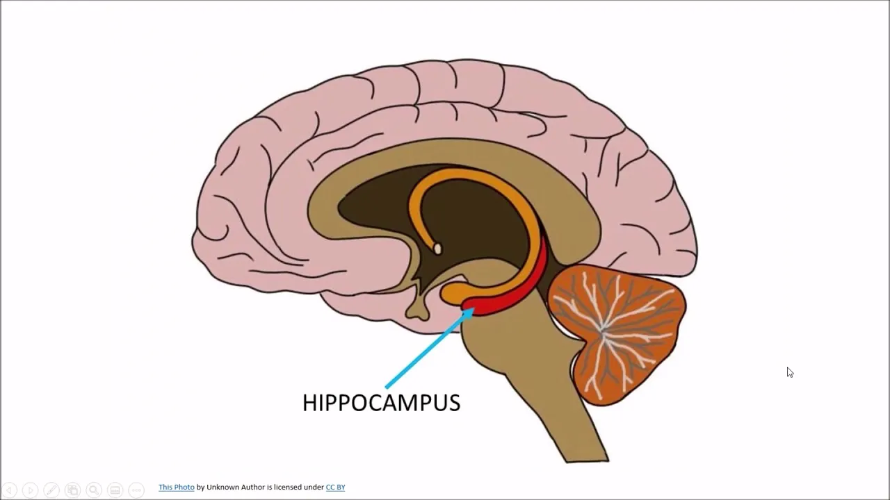
8:08
Neuroscience
What is neurodegeneration?
TheSheekeyScienceShow
3K views•2019-08-19
57:35
Neuroscience
IPL - Ruth Empson "Mind the Gap"
otagouniversity
251 views•2019-07-08
14:01
Neuroscience
How our body shapes our mind | Pancho Tolchinsky | TEDxNapoli
TEDx
2K views•2019-12-05
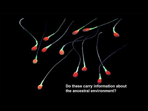
1:00:02
Neuroscience
Impact of Early Life Deprivation Danielle Stolzenberg Marcus Pembrey Bruce McEwen
uctv
4K views•2019-12-01
10:32
Neuroscience
β-Caryophyllene for Parkinson’s: Protecting Dopamine & Easing Symptoms
parkinsonsdiseaseeducation
6K views•2025-08-09

20:44
Neuroscience
New Insights from Inside the Brain with Rodrigo Braga, PhD
NUFeinbergMed
421 views•2025-04-14
9:57
Neuroscience
Highlights for dystonia • 2025 MDS Congress
movedisorder
145 views•2025-10-27

58:17
Neuroscience
Animal Welfare Synergy Series: Dr Tom Smulders on hippocampal neurogenesis
costactionlift
135 views•2025-07-14
Trending

13:25
Business
Playstation NO DISC/NO BUY Fight Is Over...
DavidJaffeGames
4K views•2026-07-23

22:40
Business
Steam and Xbox Just Dropped The Hammer On PlayStation
OhNoItsAlexx
9K views•2026-07-23

16:52
Anthropology
Americans Confused in Australia for 17 Minutes Straight
IWrocker
17K views•2026-07-23

20:36
Business
SuperBike Factory Has Gone... What's Next for the Motorcycle Industry?
thatbikersimon
11K views•2026-07-22